
Welcome to this presentation of the draft for the opening chapter of my upcoming book, titled "Structural Engineering: Dynamics, Seismic Solution, and AI Integration." This chapter delves into the intricate realm of undergraduate structural dynamics. This endeavor is not meant to mirror the exhaustive details laid out in some of the field's seminal literature. If you're familiar with works from esteemed authors such as Chopra, Mario Paz, Cloth & Penzien, among others, you'll be aware of the profound depth and rigor they bring to the underlying concepts and mathematical foundations of structural dynamics. Rather than merely echoing their profound insights, this book and the initial chapter provided here chart a distinctive course.
The chief aim is to distill intricate theoretical mathematics into more accessible discrete mathematical frameworks, offering clear outlines of pivotal concepts in dynamic structures. This proves indispensable for students traversing the expansive realm of structural dynamics. By intertwining essential theories with illustrative Python code samples, readers will unlock understanding of the fundamental mechanics underpinning both single-degree-of-freedom SDOF and multi-degree-of-freedom MDOF dynamic systems. The focus remains unwaveringly on applications within structural engineering, positioning this as a prized asset for those immersing themselves in the field. It's vital to understand that this draft of the initial chapter isn't designed to serve as an isolated guide. Instead, it acts in tandem with conventional educational tools, reinforcing the bedrock knowledge students garner in academic settings. For a nuanced and comprehensive grasp of the domain, turning to the venerable tomes of dedicated structural dynamics literature is imperative. When combined with in-depth classroom learning, the revelations from such extensive studies will unquestionably refine a scholar's proficiency. I invite you to join me on this illuminating expedition, and I hope it lays the foundation for your scholastic and professional achievements in structural dynamics.
The study of vibration phenomena in mechanical systems dates back to ancient times, but it wasn't until the 17th century that the mathematical foundations for analyzing these phenomena were developed by mathematicians such as Galileo Galilei and Isaac Newton. In the following centuries, the study of vibration became increasingly important as it was applied to practical engineering problems such as the design of machines, buildings, and bridges. One of the key developments in the analysis of vibrating systems was the discovery of the principle of superposition, which states that the response of a system to multiple excitations can be obtained by summing the responses to each excitation individually. Another important development was the realization that many practical vibrating systems can be modeled as discrete, 1-degree-of-freedom (SDOF) systems. In the 19th century, the French mathematician Joseph Louis Lagrange developed a powerful tool for analyzing the dynamics of mechanical systems, which became known as Lagrangian mechanics. This approach allows the equations of motion for a system to be derived from a single function, the Lagrangian, which describes the system's kinetic and potential energy.
Using Lagrangian mechanics, it is possible to derive the equation of motion for a discrete SDOF vibrating system. This equation relates the displacement of the system to the external forces acting on it and the system's characteristics such as its mass, stiffness, and damping. The equation can then be solved to obtain the system's displacement response to a given excitation. Today, the equation for solving the displacement response of a discrete SDOF conservative vibrating system is a fundamental tool in structural engineering and is used in many applications such as the design of buildings, vehicles, and machines. Its development represents a significant milestone in the history of vibration analysis and has paved the way for further advances in the field.
In the 18th century, Daniel Bernoulli introduced the theory of string vibrations, which led to a deeper understanding of harmonic vibrations and their relevance in musical systems. It was an epiphanic moment when engineers and mathematicians realized that the principles behind the vibration of a string on a musical instrument could also be applied to structures like bridges and buildings. This connection between music and mechanics resulted in the development of structural acoustics, a discipline that examines how vibrations travel through structures and how they can be controlled or manipulated.

In the 20th century, with the advent of more advanced technologies, the need to understand and control vibrations became even more crucial. The Tacoma Narrows Bridge disaster in 1940 is a stark reminder of the importance of considering vibrations in engineering. Due to its design and wind conditions, the bridge entered a destructive dynamic magnification, leading to its collapse. This event reshaped the way engineers approached the study of structural dynamics, emphasizing the need to consider all possible forms of excitation and response. Besides theoretical advances, there were a slew of tools and techniques that evolved to measure and analyze vibrations. For instance, Spectral Analysis allowed engineers to break down complex vibrations into their fundamental components, facilitating a better understanding and control of dynamic systems. Tools like the spectroscope and modal analysis techniques became indispensable in labs and industrial applications, enabling safer and more efficient designs.
As technology progressed into the latter half of the 20th century, computational tools became indispensable. Finite Element Analysis (FEA), a computational technique originating from the Ritz method and the Galerkin method, empowered engineers to model and simulate complex structures under dynamic loads. This method transformed how industries approached design, especially in aerospace and automotive sectors, ensuring structural integrity against vibrational loads without exhaustive physical testing. The onset of the space age brought about new challenges. The launch of satellites and spacecrafts necessitated an understanding of vibrations in a vacuum, with the absence of damping from atmospheric air. Engineers turned to historical texts and combined them with modern computational techniques. Remarkably, the works of luminaries like Leonhard Euler and Sophie Germain found renewed relevance in this era, proving that foundational principles, once established, can find utility across centuries.
In more recent times, with the rise of sustainable architecture and the pressing challenges of climate change, understanding the dynamic response of structures has taken on a new dimension. Modern buildings, such as the Taipei 101 in Taiwan, employ massive tuned mass dampers to counteract vibrations induced by earthquakes and high winds. This integration of engineering dynamics into architecture exemplifies the multidisciplinary approach of the 21st century, bridging historical knowledge with cutting-edge innovation.
In the mid-20th century, a groundbreaking discovery in the field of structural dynamics was made. Engineers developed the concept of "modal analysis," a technique that allows them to determine the natural frequencies and mode shapes of a structure. This breakthrough not only revolutionized the way we design buildings and bridges. The intersection of art and science has also been profoundly impacted by vibration analysis. In the realm of music, the study of harmonic vibrations led to the creation of musical instruments with exceptional tonal quality. Stradivarius violins, for example, are celebrated for their unique resonance properties, which remain a subject of fascination and study among both musicians and engineers. Moreover, another fascinating historical fact is the role of vibrations in the world of paleontology. By analyzing the vibrations produced by fossils, researchers can gain insights into the structure and behavior of prehistoric creatures. This interdisciplinary approach has shed light on the movements of dinosaurs and ancient marine life, adding a new dimension to our understanding of Earth's history.
In recent decades, the development of "smart materials" has brought about a paradigm shift in vibration control. Materials with the ability to adapt their stiffness and damping properties in real-time have enabled structures to actively mitigate vibrations. This innovation has found applications in skyscrapers, where sensors and actuators work together to counteract the swaying caused by high winds, ensuring occupant comfort and safety.

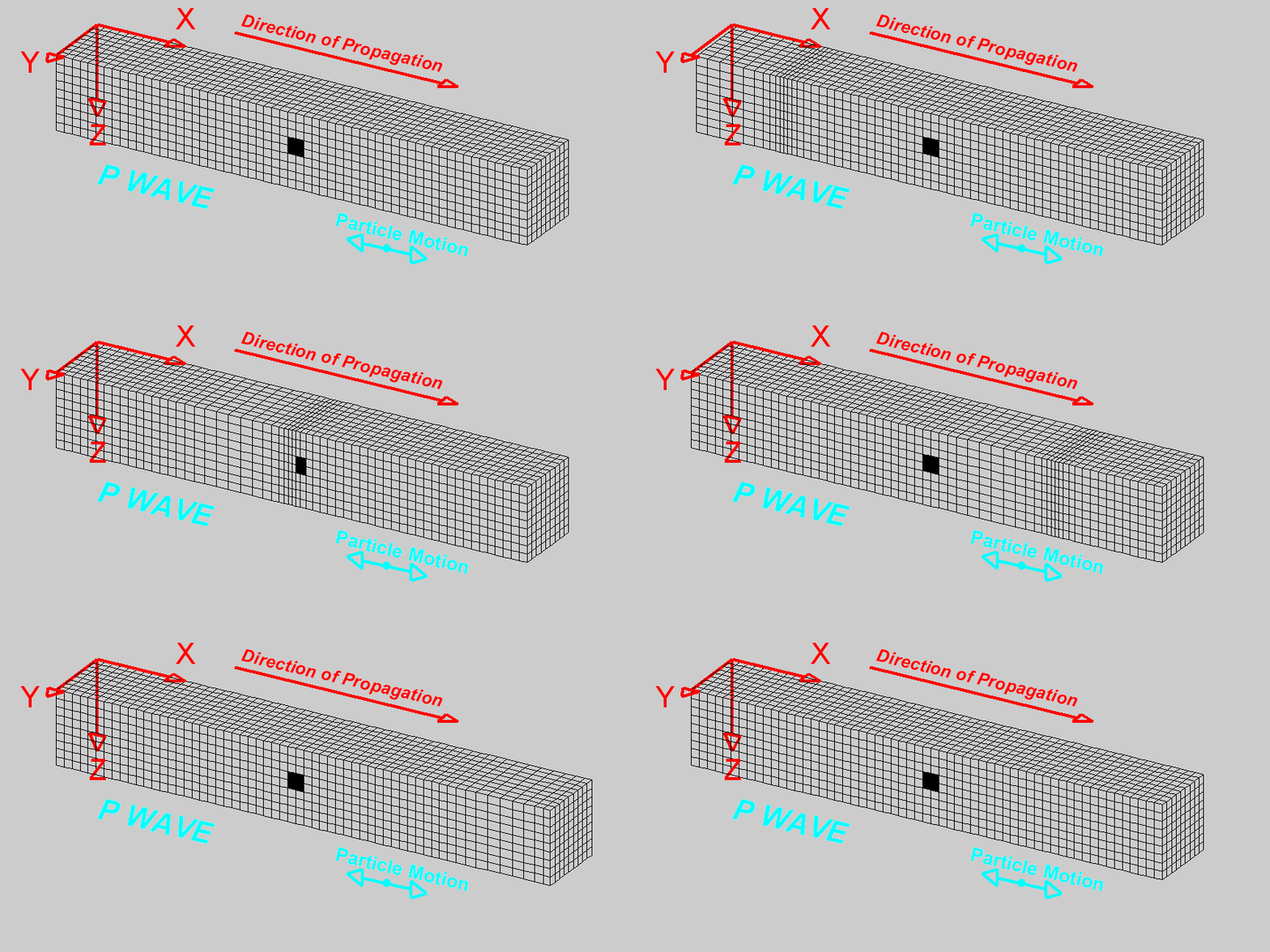
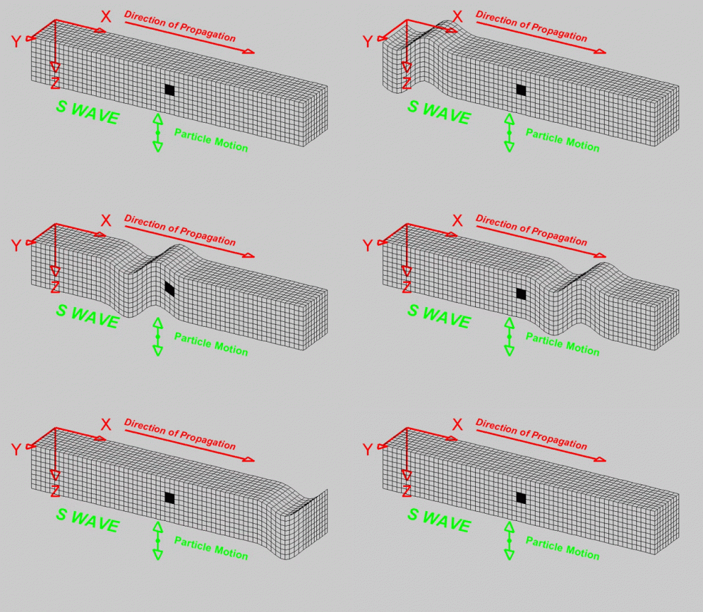
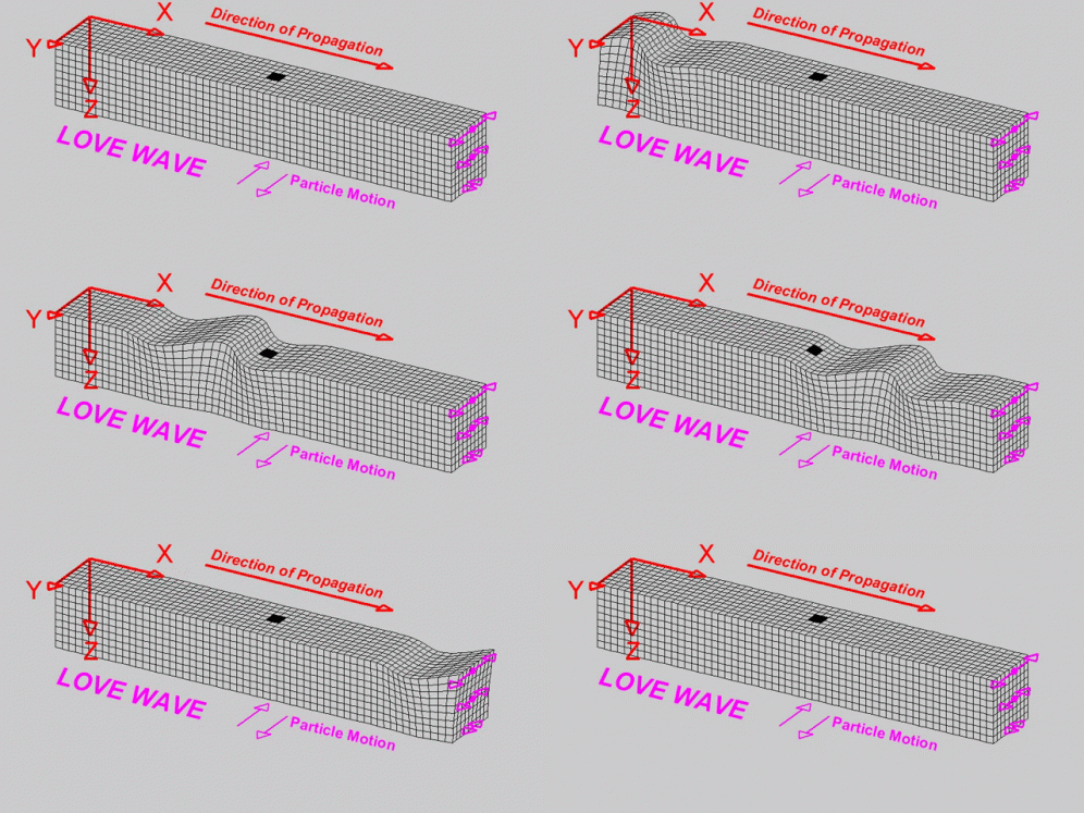
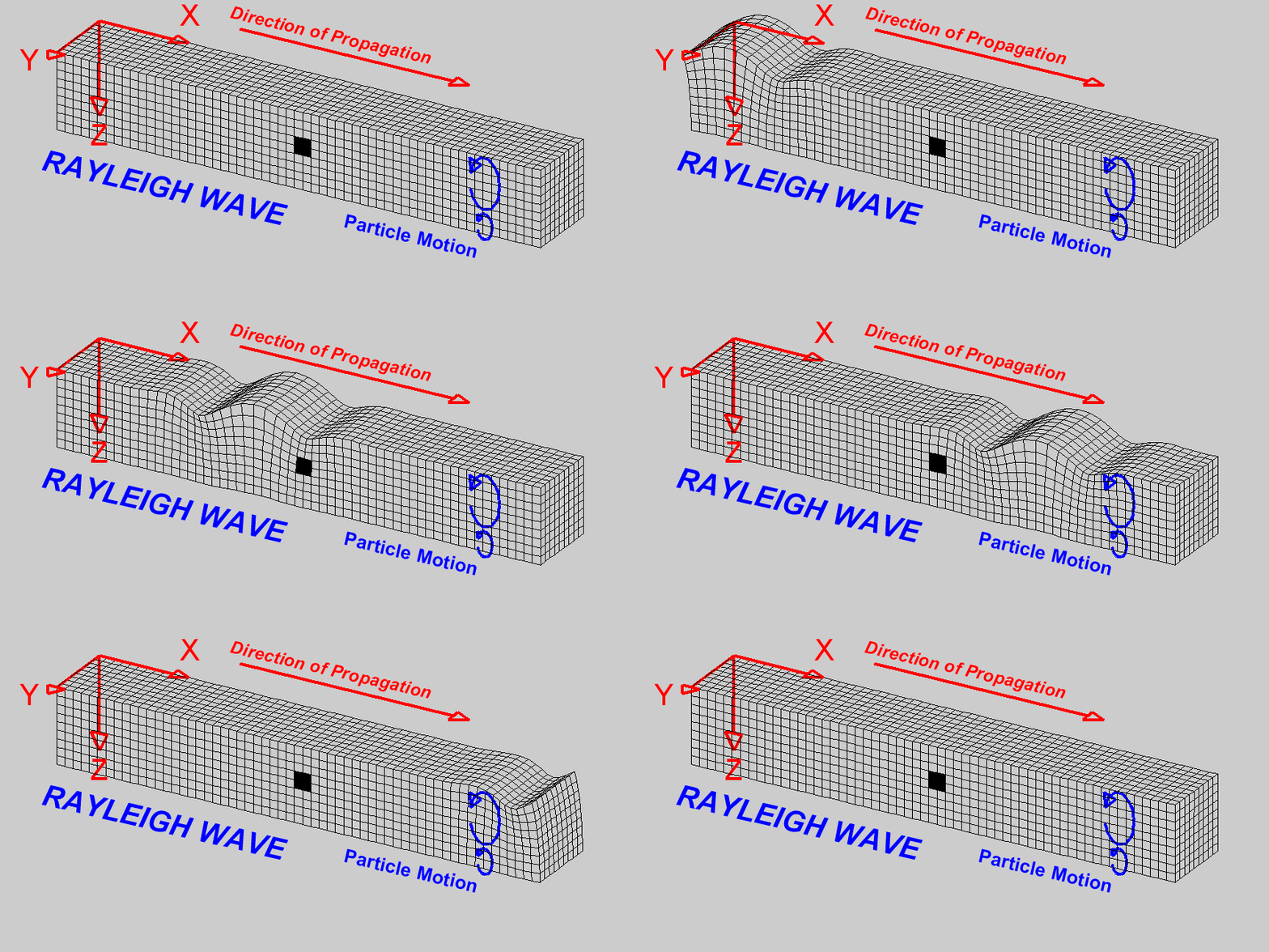
Understanding dynamic systems plays a pivotal role in seismic engineering. Just as a physician must understand human anatomy to diagnose ailments, a seismic engineer needs to grasp the interplay between a structure and the ground it's built upon. This intricate relationship, often termed soil-structure interaction (SSI), is paramount. When seismic waves traverse the Earth's layers, they don't merely dissipate upon reaching built structures. Instead, they transfer energy, leading to vibrations or, in extreme cases, severe structural damage. Owing to the Earth's layered composition, seismic events generate multiple types of seismic waves. Among the most crucial are P-waves (Primary waves) and S-waves (Secondary waves). P-waves, being compressional, can travel through both solids and liquids, making them faster and the first to be detected by seismographs. In contrast, S-waves, being shear waves, only traverse solids, rendering them slower but also more destructive due to their larger amplitudes. To assess the potential seismic impact on structures, engineers often turn to response spectrum analysis. This methodology doesn't directly consider actual earthquake time histories but instead focuses on the maximum responses of oscillators (or idealized structures) to those earthquakes. By understanding how different oscillators (representing various structural periods) respond to seismic waves, engineers can anticipate potential structural behaviors during real-life seismic events. In the modern era, with the aid of computational tools, Finite Element Methods (FEM) allow engineers to simulate complex scenarios of soil-structure interaction. These simulations take into account various soil properties, foundation depths, and structural attributes. Through iterative testing in a virtual environment, optimal designs that can withstand anticipated seismic activities in specific regions are achieved. However, while our tools and methodologies have advanced, the foundational principles remain rooted in understanding the dynamics of systems and the seismic waves generated by the Earth. Recognizing the unique characteristics of P-waves, S-waves, and even surface waves ensures that structures are not just built to stand tall but also to sway and oscillate in harmony with the Earth's rhythms, thus ensuring safety and longevity.'
Animation Source: NOA
In order to establish a solid foundation for understanding the terminology related to structural dynamics used throughout this document, it's essential to be acquainted with the foundational concepts. These help in grasping the vibrations of systems and, by understanding them, we can make predictions regarding their behavior. It's crucial to understand that while seismic phenomena fall within the realm of dynamics, the concept of "prediction" isn't directly applicable due to their non-harmonic and non-periodic nature. However, grasping the dynamic behavior of seismic events from a probabilistic perspective is indispensable in structural design. As previously mentioned, the response of structural systems to such external excitations can currently be represented both mathematically and computationally with reasonable accuracy.
Note: Additional concepts will be elaborated upon as needed or when context expansion is required throughout the document.
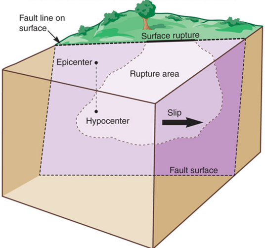
Note: Faults can manifest in different ways.
Animation Source: J.Ziony, ed. “Earthquakes in the Los Angeles Region.” USGS.

Animation Source: Seismological Facility for the Advancement of Geoscience
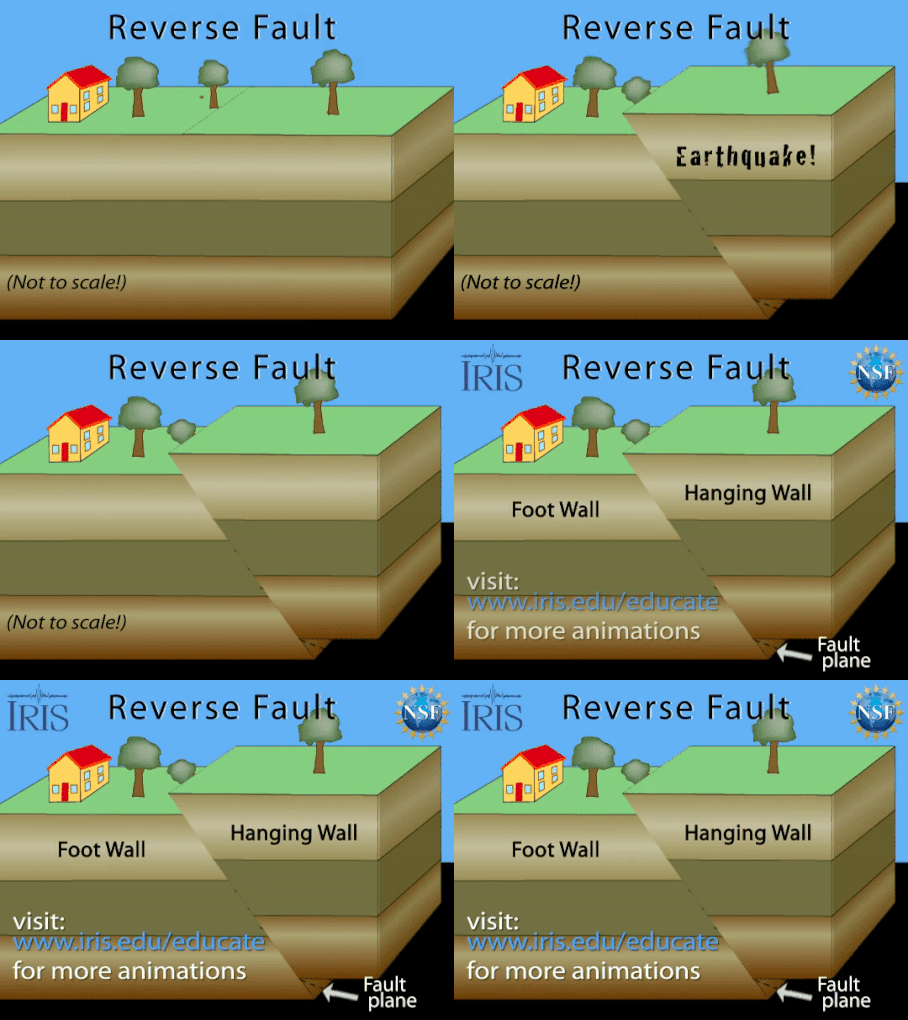
Animation Source: Seismological Facility for the Advancement of Geoscience
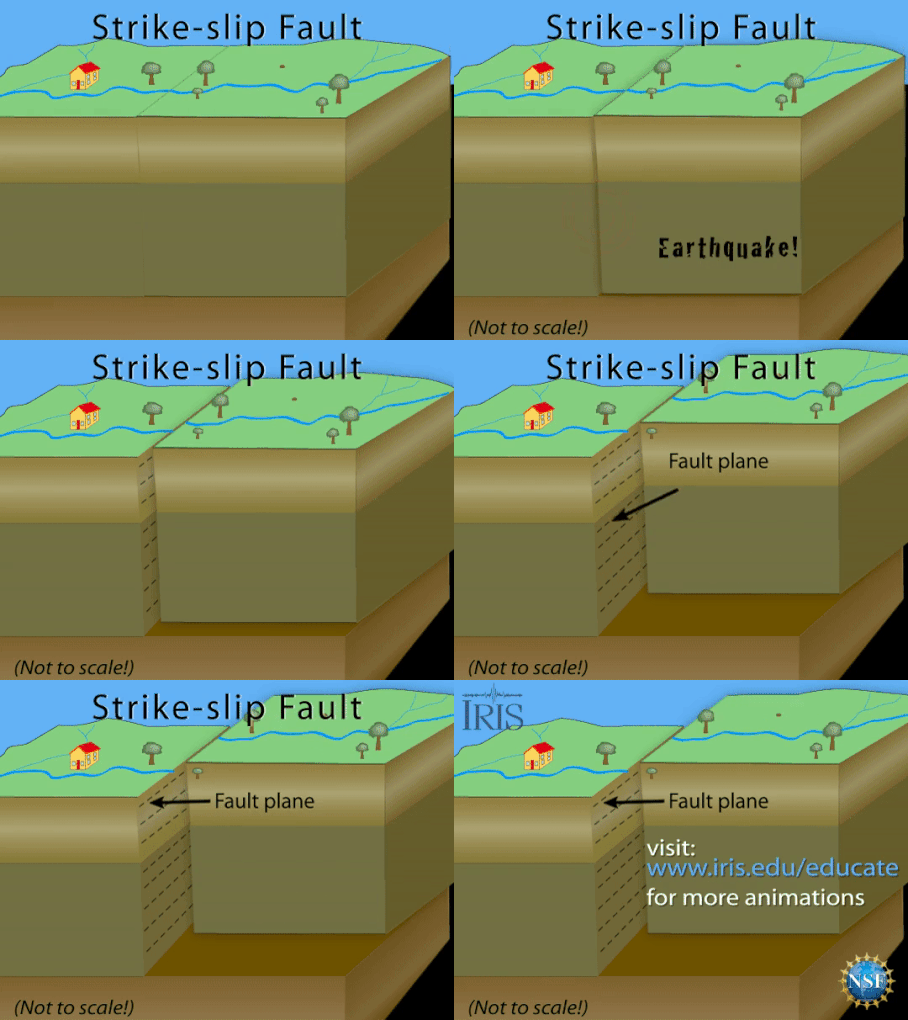
Animation Source: Seismological Facility for the Advancement of Geoscience

Animation Source: California Intitude of Technology
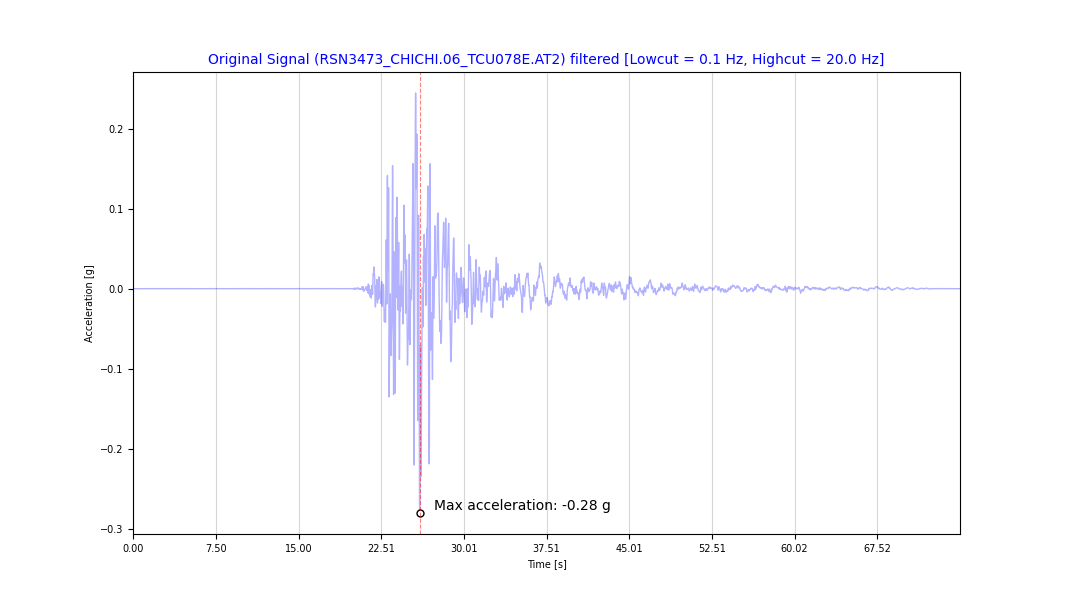
Seismic Accelerogram: A record that depicts the variation of ground acceleration with respect to time during an earthquake. It provides valuable data about the intensity and characteristics of seismic waves as they pass through a specific location.
Note: Seismic events propagate in the form of waves, and, like waves in any elastic medium, they undergo phenomena such as reflection, refraction, polarization, diffraction, dissipation and attenuation. Because these waves traverse the layers of the Earth and its discontinuities, they generate new waves that complicate the interpretation of seismic records. Due to this, seismic waves can be highly variable; however, they can be classified into families, which will be described below.

System: Is a set of components with specific properties that respond to external excitation by vibrating.
Discrete System: A system where the physical properties of its components are distinctly localized or concentrated at clearly identified points or positions. Contrary to continuous systems where properties are distributed over a spatial extent, discrete systems, often represented by a finite number of degrees of freedom, are typically described using algebraic equations or ordinary differential equations (ODEs).
Consider, for instance, a mass-spring system with a finite number of masses and springs, which serves as a classical example of a discrete system. In such systems, the dynamics of each component can typically be defined using a set of differential equations based on Newton’s second law.
Continuous System: A system wherein the physical properties are distributed throughout its extent, rather than concentrated at discrete points. Unlike discrete systems, continuous systems are described using field variables which vary over space, typically represented using partial differential equations (PDEs).
A foundational example of a continuous system is a stretched string or beam. The vibration of such a system is described by the wave equation:
$$ \frac{\partial^2 u(x,t)}{\partial t^2} = c^2 \frac{\partial^2 u(x,t)}{\partial x^2} $$Where:

Video Source: Jason Bramburger
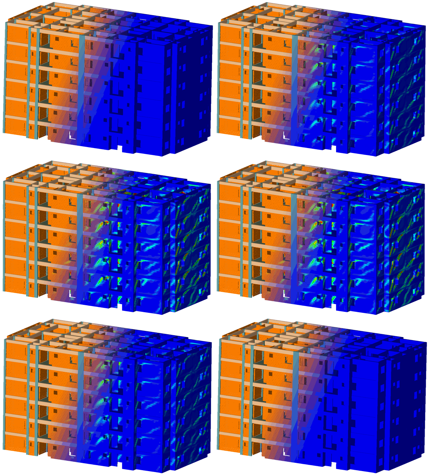
External Excitation: External action that induces vibration in a system.
Impulsive Dynamic Excitation: An external action that varies with time and is completely independent of the system's motion.
Dynamic Impact Excitation: An external action that varies with time and depends on the motion of the system.
Response: Displacement, speed, or acceleration outcomes in a system's vibration, resulting from external excitation or free vibration.
Animation Source: Extreme Loading for Structures
Animation Source: FREEform

Animation Source: Flipping Physics
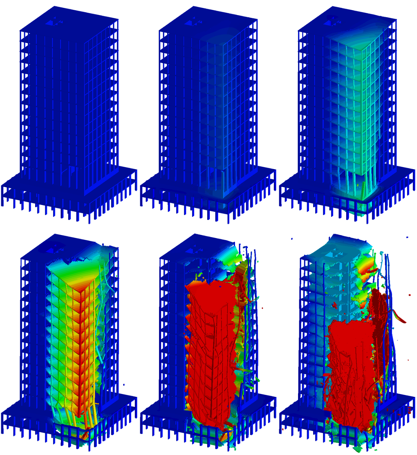
Dynamic Analysis: A study centered on understanding the forces and motions of systems over time, particularly those in free vibration or subjected to external excitation. (Structural Dynamics).
Deterministic Dynamic Analysis: A dynamic analysis that assumes complete knowledge of the external excitation in the time domain.
Probabilistic Dynamic Analysis: This refers to a method used in engineering, especially in the realm of structural engineering, to assess the response of a system under dynamic loads by considering the uncertainties inherent in the system properties, external loads, and initial conditions. Instead of analyzing a single deterministic scenario, probabilistic dynamic analysis evaluates multiple scenarios considering the probabilistic distribution of various input parameters.
Key points:
Stochastic Modeling: The inherent randomness of certain parameters (like material properties, loads, and boundary conditions) is represented using probabilistic distributions.
System Response: The analysis yields probabilistic descriptions of the system response instead of deterministic single values.
Risk Assessment: By understanding the probabilistic nature of the system's response, one can make more informed decisions regarding safety, reliability, and performance.
Animation Source: Extreme Loading for Structures

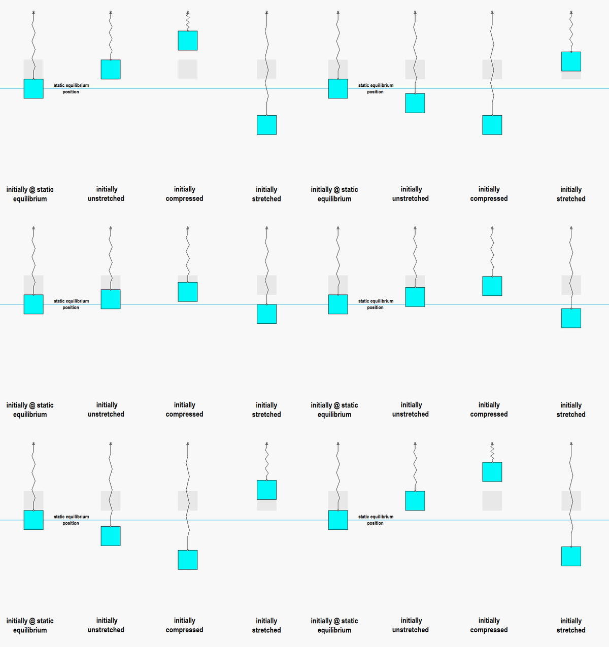
Vibration: Refers to the oscillatory motion of a system about an Static Equilibrium Position.
Free Vibration: The natural oscillation of a system in the absence of external forces.
Forced Vibration: Oscillation that occurs when an external force is applied to a system, driving it to vibrate at the frequency of the applied force, potentially leading to dynamic magnification if the forcing frequency is close to the system's natural frequency.
Vibration Cycle: One complete motion or oscillation of a vibrating system from its initial position, through its maximum displacement, and back to its initial position.
Periodic Motion: A motion that repeats itself in regular intervals of time, characterized by a definitive period or frequency.
Animation Source: Wikipedia

Vibration Period [T]: The time taken for a vibrating system to complete one full cycle of its motion, from a specific point back to the same point. It's essential to understand that for a vibration cycle, and consequently a vibration period, to exist, the system must be considered conservative, implying no energy is lost over time. is typically measured in Seconds (s)
Vibration Frequency [f]: The number of cycles of vibration that occur in one second. It is the reciprocal of the vibration period "$ f = \frac{1}{T} $" and is typically measured in Hertz (Hz).
Animation Source: Wikipedia
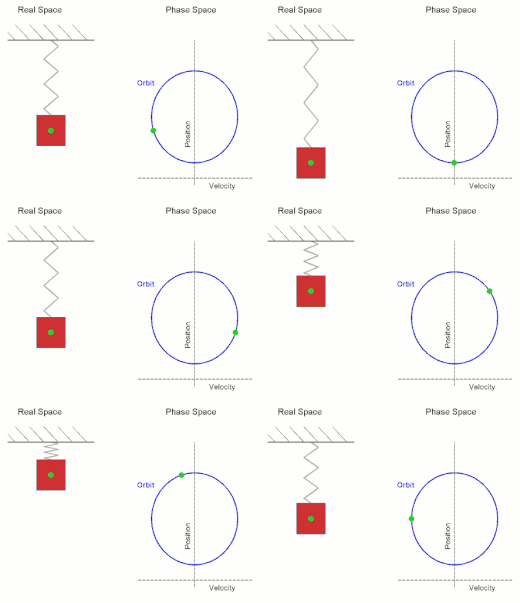
Simple Harmonic Motion (SHM): A type of periodic motion where an object moves back and forth about a central position due to a restoring force proportional to its displacement from the equilibrium. The trajectory of this motion follows a sinusoidal path, making it describable by sine and cosine functions.
Dynamic Degree of Freedom: Refers to the number of independent ways a dynamic system can move without violating any constraint imposed upon it. In essence, it determines the minimum number of independent coordinates required to describe the motion or configuration of the system at any given time.
Inertial Reference Frame: A frame of reference in which Newton's first law of motion (the law of inertia) holds true. In such a frame, an object not subject to external forces will remain at rest or move at a constant velocity. Non-inertial reference frames, on the other hand, are accelerating and therefore, experience fictitious forces.
Animation Source: Wikipedia
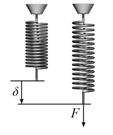
Stiffness: In structural engineering and mechanics, stiffness refers to the extent to which an object or material resists deformation in response to an applied force. It's quantified as the ratio of the force applied to the deformation produced (Hooke's law). In terms of structures, stiffness often determines how much a structure will deform or deflect under specific loads. Mathematically, for linear elastic materials, stiffness $ K $ is described by the equation:
$$ P = K \cdot \delta $$Where:
Animation Source: Wikipedia
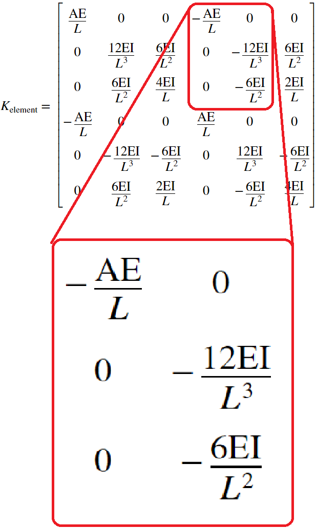
Stiffness Coefficients: These are constants that quantify the resistance of structural elements to deformation when subjected to forces. They often represent the linear relationship between force and displacement for a specific degree of freedom in a structural system.
Stiffness Matrix: A square matrix used in structural element analysis that relates nodal displacements to nodal forces within a structure or a structural element. Each entry in the matrix represents the reaction force induced at a node for a unit displacement imposed at another node, while keeping all other nodes restrained. This matrix encapsulates the structural behavior of the element or the entire system under study. For a linear elastic system, the relationship between forces $ P $ and displacements $ \delta $ can be represented as:
$$ \lbrace P_{\scriptstyle \text{GDLg}} \rbrace = [K]_{\scriptstyle \text{GDLg}} \cdot \lbrace \delta \rbrace_{\scriptstyle \text{GDLg}} \rightarrow \lbrace \delta \rbrace_{\scriptstyle \text{GDLg}} = [K]_{\scriptstyle \text{GDLg}}^{-1} \cdot \lbrace P_{\scriptstyle \text{GDLg}} \rbrace $$
Where:
Animation Source: Author's own.

Damping: A phenomenon in which the energy of an oscillating system decreases over time, usually due to the conversion of mechanical energy into heat or other forms of energy. Damping tends to reduce the amplitude of oscillations and can bring an oscillating system to rest if there is enough of it.
Equivalent Viscous Damping ($ c $): A conceptual form of damping used to describe the energy dissipation characteristics of a system in terms equivalent to those of a viscous damper. It's often used in structural engineering and earthquake engineering to relate actual complex damping mechanisms to a simpler linear damping model, enabling the use of standard analysis techniques.
Damping Factor ($\xi$): A dimensionless quantity used to describe the amount of damping in a system relative to critical damping. It provides a measure of the energy dissipated in an oscillatory system. A system with $\xi$ = 0 is undamped, while $\xi$ = 1 represents a critically damped system. Values between 0 and 1 indicate underdamping, and values greater than 1 indicate overdamping.
Animation Source: Wikipedia
Animation Source: Author's own.

Weight: The gravitational force exerted on an object due to the mass of the object and the acceleration due to gravity. It is a vector quantity, meaning it has both magnitude and direction, and it always acts downward towards the center of the Earth (or any other massive body).
Elastic Force: A restoring force that acts to bring a system back to its equilibrium position. It is directly proportional to the displacement of the system from its equilibrium position, especially as described by Hooke's law in many materials.
Video Source: Veritasium

Newton's Laws of Motion: These fundamental principles, articulated by Sir Isaac Newton in his work "Philosophiæ Naturalis Principia Mathematica" in the 17th century, provide the foundation for classical mechanics, describing the relationship between the forces acting on a body and its motion. The laws are as follows:
First Law (Law of Inertia): A body will preserve its state of rest or of uniform motion in a straight line unless it is compelled to change that state by forces acting upon it. This is a manifestation of the inertial property of matter. It introduces the concept of inertia and serves as a statement of what happens in the absence of net external forces.
Second Law (Law of Acceleration): The net force acting on an object is directly proportional to the rate of change of its momentum. For objects with constant mass, this relationship simplifies to:
Where:
$ F $: represents the net external force acting on the object.
$ m $: is the system mass.
$ a $: is its acceleration. The direction of the acceleration is the same as the direction of the net force.
Note: It's essential to underscore that the equation previously mentioned embodies the essence of Newton's second law. This law is characterized by a second-order ordinary differential equation.
Animation Source: Wikipedia

$$ F_{external} - m \cdot a = 0 $$
Where:
$ F_{external} $ : is the external force acting on the system, "$ m $" is the mass of the system, and "$ a $" is its acceleration. The term "$ -m \cdot a $" is often referred to as the "D'Alembert force" or "inertial force".
Animation Source: Wikipedia
Differential Equation of Dynamic Equilibrium: The core principle behind this equation is the conservation of energy in dynamic systems, specifically addressing how energy is distributed among various forms: potential, kinetic, and dissipative due to damping. Rooted deeply in the laws of motion and energy conservation, it's the mathematical formulation that captures the dynamic behavior of systems subjected to time-varying external forces or initial conditions.
At any given instant of time, the sum of the inertial forces (proportional to acceleration), damping forces (proportional to velocity), and elastic (or restoring) forces (proportional to displacement) in the system must equal the externally applied forces. Mathematically, this relationship can be captured by the equation:
$$ m \ddot{x}(t) + c \dot{x}(t) + k x(t) = f(t) $$Where:
The equation encapsulates a balance where the sum of inertial, damping, and restoring forces within the system equals the external forces acting upon it. This balance, inherently a manifestation of Newton's second law in dynamic contexts, provides foundational understanding and predictive capability in various engineering, physical, and scientific applications.

Beyond the foundational definitions provided earlier, it's imperative to delve deeper into the mathematical framework underlying the behavior of structural systems in both free and forced vibrations systems. A foundational approach to comprehending this intricate behavior begins with the most elementary mathematical representation: The Simple Harmonic System. Is fundamentally anchored in an un-damped Single Degree of Freedom SDOF system, characterized by a consistent angular velocity $(\omega_n)$.
The mathematical derivation of this system is firmly rooted in two primary principles. First, the principle of energy conservation, which dictates that the total energy in an isolated system remains unchanged over time. And second, the foundational concept of constant velocity, which, in its simplest form, is expressed as the ratio of distance traveled to the time taken.
While many educational settings have likely introduced and dissected the mechanics of this topic, a comprehensive understanding requires a deeper dive into its intricate nuances. In the ensuing discussion, we will elucidate the pivotal equations borne from the study of simple harmonic motion. Furthermore, we will explore the applications of these equations, demonstrating how they can be adeptly used to predict a system's position, velocity, and acceleration when its initial conditions are known. It's paramount to emphasize that these mathematical formulations, although insightful, are based on the simplified analogy of a conservative discrete SDOF system. Consequently, while they offer significant insights, they also come with inherent constraints and limitations that one must be cognizant of.
Delving deeper into the realms of the Simple Harmonic System, it becomes evident that its mathematical elegance and simplicity have profound implications for the real-world understanding of dynamic systems. The SDOF model, albeit an idealization, paves the way for understanding more complex systems by isolating the essential physics of vibrations. The inherent beauty of the Simple Harmonic System lies in its cyclical nature, represented by sinusoidal functions. These functions not only describe the system's position over time but also elegantly encapsulate the fundamental attributes of periodic motion, including amplitude, frequency, and phase. The angular frequency $(\omega_n)$ is particularly noteworthy, as it signifies the natural frequency of the system — a unique attribute dependent solely on the system's stiffness and mass. This frequency underscores the system's propensity to oscillate at a characteristic rate in the absence of external influences, a concept that resonates deeply with the intrinsic rhythmic patterns observed in nature and engineered structures alike.
Building upon these principles, the mathematical representation of the system evolves into a second-order differential equation, typically known as the equation of motion. This equation, derived from Newton's second law, correlates the net force acting on the system with its acceleration, factoring in both the restoring force due to the system's stiffness and the inertial force due to its mass. Herein lies the crux of understanding dynamic behavior (the interplay between force and response, cause and effect, that governs oscillatory motion). However, the real world rarely adheres to the simplifications of an idealized SDOF system. Real systems exhibit damping, a phenomenon where energy is dissipated over time, typically in the form of heat, altering the pristine sinusoidal responses predicted by the simple harmonic model. Damping brings forth the concept of the damped natural frequency, a slightly altered version of the natural frequency, accounting for the energy dissipated with each cycle of motion. The consideration of damping is not merely an academic exercise; it is a critical component in the design and analysis of systems, especially when assessing their responses to dynamic loading, such as in seismic or wind engineering.
Furthermore, one must consider the influence of external excitations. These are forces that are not accounted for within the conservative system model but are crucial for understanding the behavior of structures under operational or environmental loads. In engineering practice, these excitations often manifest as harmonic, periodic, or even random forces or non periodic non armonic exitations, each with its own set of analytical challenges. In essence, while the Simple Harmonic, Undamped SDOF System provides a valuable foundation, it is the springboard from which we dive into the rich, intricate world of vibrations in real systems. From the exploration of these concepts emerges a more comprehensive, nuanced understanding of dynamic systems, illuminating both their predictable simplicity and captivating complexity. However, as we venture into these complexities, we must remain anchored in the fundamental principles, appreciating the insights they offer while navigating the vast ocean of nuances that define real-world dynamic behavior.
Note: You can find more information in the recommended bibliography. Additionally, further digital resources on the topic are available here.
In classroom settings, it's often encouraged to meticulously unpack the mathematical underpinnings of Simple Harmonic Motion (SHM). While we won't traverse the entire deductive journey here, we'll highlight key equations and insights. A core tenet to grasp is that for a conservative SDOF discrete system (as described in Section 1.2), the angular velocity or angular frecuency, denoted $\omega_n$, remains unchanging. This constancy implies that any shift in the circular trajectory of motion can be derived from its spatial rate of change over time.
A full cycle of this movement, termed "vibration", depicted in the associated figure, accounts for a $2\pi$ displacement. Given this, the time it demands to complete one full cycle becomes $\frac{2\pi}{\omega_n}$. In simpler terms, the system's vibrational period is expressed as $T = \frac{2\pi}{\omega_n}$. To further comprehend this, consider the foundational principles of trigonometry and geometry. When applied to the figure provided, they allow us to dissect the angular movement's projection onto its Cartesian counterparts. This application is pivotal both when assessing the system's outset position $x_0$, and when pinpointing its location at any subsequent time, represented as $x(t)$.
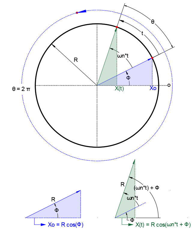
$$ \omega_n $$ $$ \theta = \omega_n \times t $$ $$ x_0 = R \cdot \cos(\phi) $$ $$ x(t) = R \cdot \cos(\omega_n \times t + \phi) $$ $$ \dot{x}(t) = -R \cdot \omega_n \cdot \sin(\omega_n \times t + \phi) $$ $$ \ddot{x}(t) = -R \cdot \omega_n^2 \cdot \cos(\omega_n \times t + \phi) $$ $$ T = \frac{2\pi}{\omega_n} $$ $$ f = \frac{1}{T} = \frac{\omega_n}{2\pi} $$ $$ \omega_n = \frac{2\pi}{T} $$ $$ R = \sqrt{x^2 + \frac{\dot{x_0}^2}{\omega_n^2}} $$ $$ \phi = \arctan\left(-\frac{\dot{x_0}}{\omega_n x_0}\right) $$ $$ x(t) = R \cdot \cos(\omega_n \times t + \phi) \ \ \boldsymbol{\color{blue}{\xRightarrow{\hspace*{0.7cm}{}}}} \ \ \boxed{x(t) = x_0 \cos(\omega_n t) + \frac{\dot{x_0}}{\omega_n} \sin(\omega_n t)} $$
Where:
$ \omega_n $: Angular Velocity or Angular Frequency
$ \theta $: Angular displacement
$ x_0 $: Initial position
$ x(t) $: Position as a function of time
$ \dot{x}(t) $: First derivative of position with respect to time (velocity)
$ \ddot{x}(t) $: Second derivative of position with respect to time (acceleration)
$ T $: Period
$ f $: Frequency
$ R $: Amplitude
$ \phi $: Phase angle
Underdamped single-degree-of-freedom discrete systems are commonly used to model mechanical systems, such as springs and masses, that undergo vibration. These systems can be described by second-order linear differential equations, which can be solved using various methods, including analytical and numerical approaches. Equations are particularly useful for solving these systems because they allow us to predict the behavior of the system over time without having to perform physical experiments. Equations can also be used to analyze the system's response to different inputs, such as initial conditions or external forces.
To solve the equation of motion for an underdamped single-degree-of-freedom system, we typically use the characteristic equation and the associated damping ratio to determine the system's natural frequency and frequency of damped oscillation. From there, we can derive equations for the system's displacement, velocity, and acceleration over time.
The equation of motion for a sub-damped single degree of freedom discrete conservative system subjected to a free vibration can be expressed as:
$$ m\ddot{x}(t) + c\dot{x}(t) + kx(t) = 0 $$
where:
$m$ ,is the mass of the system
$k$ ,is the stiffness coefficient
$x(t)$ ,is the displacement of the system
The natural frequency of the system can be calculated as:
$$ \omega_n = \sqrt{\frac{k}{m}} $$
where $\omega_n$, is the natural frequency.
The damping ratio can be calculated as:
$$ \zeta = \frac{c}{2\sqrt{km}} $$
where $\zeta$, is the damping ratio.
The period of the system can be calculated as:
$$ T = \frac{2\pi}{\omega_n} $$
where $T$, is the time period.
The general solution of the equation of motion can be expressed as:
$$ x(t) = e^{-\zeta\omega_n t}(C_1\cos(\omega_d t) + C_2\sin(\omega_d t)) $$
where:
$C_1$ and $C_2$ are constants determined by initial conditions $\omega_d = \omega_n\sqrt{1-\zeta^2}$ is the damped natural frequency.
The initial conditions can be defined as:
$x(0) = x_0$, initial displacement $\dot{x}(0) = v_0$, initial velocity
The constants $C_1$ and $C_2$ can be calculated using the initial conditions:
$$ C_1 = x_0 $$ $$ C_2 = \frac{\dot{x}(0) + \zeta\omega_n x_0}{\omega_d} $$
By applying the above equations, the response of a sub-damped single degree of freedom discrete conservative system subjected to a free vibration can be calculated.
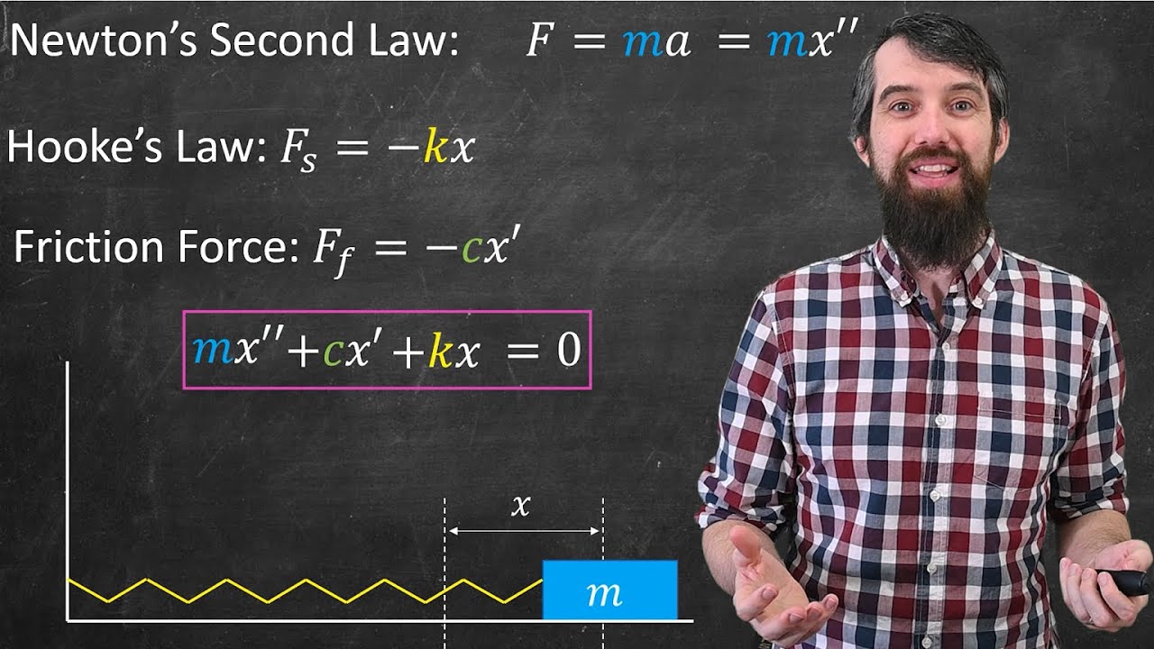
If you want to find more information about the response of SDOF underdamped discrete systems, you can access the following two links:

Video: "Introduction to Dynamics" [Physics for Everyone].
(2022, April 15). Retrieved from https://www.youtube.com/watch?v=vLaFAKnaRJU
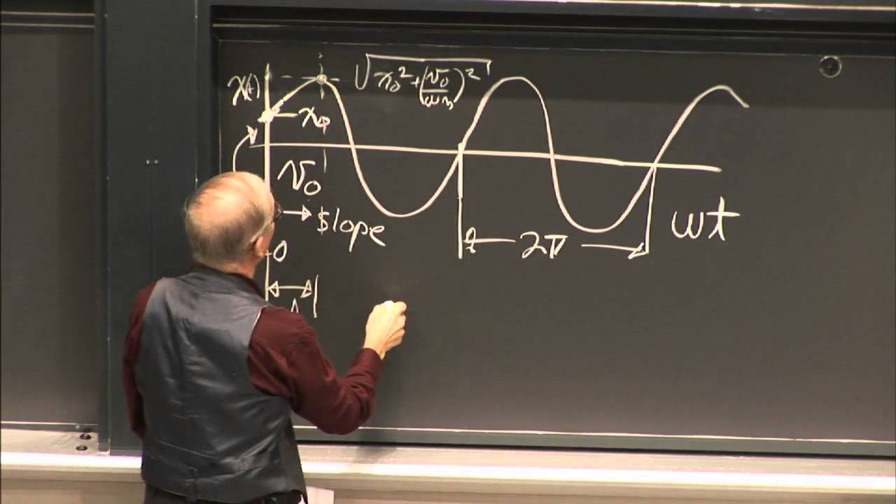
Video: "Introduction to Classical Mechanics" [MIT OpenCourseWare].
(2013, September 2). Retrieved from https://www.youtube.com/watch?v=CTd1uVq5-l8
Video: "Introduction to Mechanical Vibration" [MIT OpenCourseWare].
(2011). Retrieved from https://www.youtube.com/watch?v=9_d8CQrCYUw
import numpy as np
import pandas as pd
import matplotlib.pyplot as plt
import matplotlib.animation as animation
%matplotlib widget
Problem Data
xo = 1                                                                              # Initial displacement
xvo = 0                                                                             # Initial velocity
to = 0                                                                              # Start time
tf = 5                                                                              # End time
delta = 0.001                                                                       # Time step size
Peso = 16.25                                                                        # Weight of the system
g = 9.81                                                                            # Acceleration due to gravity
E = 2000000                                                                         # Modulus of elasticity of the system
I = 0.3**4/12                                                                       # Moment of inertia of the system
L = 2.50                                                                            # Length of the system
K = 24*E*I/L**3                                                                     # Stiffness coefficient of the system
M = Peso/g                                                                          # Mass of the system
w = np.sqrt(K/M)                                                                    # Natural frequency of the system
d = np.log(1/0.81)                                                                  # Logarithmic decrement of the system
zi = np.sqrt((d**2)/(4*np.pi**2+d**2))                                              # Damping ratio of the system
wz = w*np.sqrt(1-zi**2)                                                             # damped natural frequency
num_cicles = 6                                                                      # Maximum consecutive sought
Solution
x = []                                                                              # Displacement matrix initialization
ti = []                                                                             # Time matrix initialization

for t in np.arange(to, tf, delta):                                                  # Loop over time values
    x_t = np.exp(-zi*w*t)*(xo*np.cos(wz*t) + (xvo + w*zi*xo)/(wz)*np.sin(wz*t))     # Calculate the displacement at each time step
    ti.append(t)                                                                    # Append the time value to a list
    x.append(x_t)                                                                   # Append the displacement value to a list
maxx = []
tix = []
z=1
for z in range(len(x)):                                                             # Loop over displacement values to find maximum points
    if x[z]>x[z-1] and x[z]>x[z+1]:                                                 # Check if the displacement value is greater than its neighbors
        maxx.append(x[z])                                                           # Append the maximum displacement value to a list
        tix.append(ti[z])                                                           # Append the corresponding time value to a list
MaxX_ti = pd.DataFrame({"Time [s]": tix,"Displacement": maxx})                      # Create a pandas dataframe with maximum displacement values and their corresponding time values
MaxX_ti.head(num_cicles+1)                                                          # Show the DataFrame
| Time [s] | Displacement | |
|---|---|---|
| 0 | 0.000 | 1.000000 |
| 1 | 0.178 | 0.809950 |
| 2 | 0.355 | 0.656043 |
| 3 | 0.533 | 0.531440 |
| 4 | 0.711 | 0.430450 |
| 5 | 0.888 | 0.348638 |
| 6 | 1.066 | 0.282427 |
Figure
fig, ax = plt.subplots(figsize=(16/1.5, 9/1.5))                                                                 # Create a figure and an axes object

ax.plot(ti, x, color=(0, 0, 1), marker='+', markersize=0, markerfacecolor='w',                                  # Plot the displacement response using blue markers
 markeredgewidth=0, linewidth=1, alpha=0.5,label= f'Displacement Response, $ \zeta $  = {(zi*100):.2f} %')
ax.plot(tix[num_cicles], maxx[num_cicles], marker='o', markersize=5, markerfacecolor='black',                   # Plot the max displacement response using black marker
 markeredgewidth=0, linewidth=1, alpha=1.0)

ax.set_xlim([0, max(ti)])                                                                                       # Set the x-axis limits from 0 to the maximum value in ti
plt.title('Displacement Response', fontsize=14, color=(0, 0, 1))                                                # Set the title of the plot to 'Displacement Response'
plt.xlabel('Time [s]', rotation=0, fontsize=10, color=(0, 0, 0))                                                # Set the x-axis label to 'Time [s]'
plt.ylabel('Amplitude [X]', rotation=90, fontsize=10, color=(0, 0, 0))                                          # Set the y-axis label to 'Amplitude [X]'
ax.axvline(x=tix[num_cicles], color=(1, 0, 0), alpha=0.5,
               linewidth=0.8, linestyle='dashed')                                                               # Draw a vertical line at the x-coordinate of the maximum consecutive analysis
ax.text(tix[num_cicles]*1.05, maxx[num_cicles],
        f"Xmax_cicle_{num_cicles:.0f} = {maxx[num_cicles]:.4f}", ha='left', va='bottom', rotation=90)
legend = plt.legend(fontsize=10)                                                                                # Add a legend to the plot with a font size of 10
legend.get_frame().set_edgecolor('none')                                                                        # Remove the frame from the legend
ax.grid(which='both', axis='x', alpha=0.5)                                                                      # Add gridlines to both the x and y axis
plt.show()                                                                                                      # Show the plot
### Solution using consecutive maximums.
xmaxcicle = xo/np.exp(num_cicles*d)                                                                             # Maximum response at the selected cycle (numerical approach)
print('\x1b[1;34m  Xmax_aprox =', maxx[num_cicles], '\x1b[1;34m  Xmax_exact =', xmaxcicle)
Xmax_aprox = 0.28242711271069504 Xmax_exact = 0.2824295364810001
# fig, ax = plt.subplots(figsize=(16/1.5, 9/1.5))

# line, = ax.plot([], [], color=(0, 0, 1), marker='+', markersize=0, markerfacecolor='w',                         # create an empty line object to be updated in the animation
#                  markeredgewidth=0, linewidth=1, alpha=0.5,label= f'Displacement Response, $ \zeta $  = {(zi*100):.2f} %')
# ax.set_xlim([0, max(ti)])                                                                                       # Set the x-axis limits from 0 to the maximum value in ti
# ax.set_ylim([max(x)*-1, max(x)])                                                                                # Set the x-axis limits from 0 to the maximum value in x
# plt.title('Displacement Response', fontsize=14, color=(0, 0, 1))                                                # Set the title of the plot to 'Displacement Response'
# plt.xlabel('Time [s]', rotation=0, fontsize=10, color=(0, 0, 0))                                                # Set the x-axis label to 'Time [s]'
# plt.ylabel('Amplitude [X]', rotation=90, fontsize=10, color=(0, 0, 0))                                          # Set the y-axis label to 'Amplitude [X]'
# ax.axvline(x=tix[num_cicles], color=(1, 0, 0), alpha=0.5,
#         linewidth=0.8, linestyle='dashed')                                                                      # Draw a vertical line at the x-coordinate of the maximum consecutive analysis
# ax.text(tix[num_cicles]*1.05, maxx[num_cicles],
#         f"Xmax_cicle_{num_cicles:.0f} = {maxx[num_cicles]:.4f}", ha='left', va='bottom', rotation=90)
# legend = plt.legend(fontsize=10)                                                                                # Add a legend to the plot with a font size of 10
# legend.get_frame().set_edgecolor('none')                                                                        # Remove the frame from the legend
# ax.grid(which='both', axis='x', alpha=0.5)                                                                      # Add gridlines to both the x and y axis

# def update(i):                                                                                                  # define a function to update the line object in each frame of the animation
#     line.set_data(ti[:i], x[:i])
#     return line,

# ani = animation.FuncAnimation(fig, update, frames=len(ti), interval=50, blit=True)                              # decrease the interval time to 2ms

# ani.save('displacement_response.gif', writer='pillow')                                                          # save the animation as a gif
The history of how the equations that describe the response of a discrete, single degree of freedom, underdamped system to an external seismic excitation were discovered is a fascinating one. It all started with the study of the behavior of mechanical systems subjected to dynamic loads, which was an essential topic in engineering and physics at the time. In the early 20th century, engineers and scientists began to develop mathematical models that could describe the dynamic response of mechanical systems to seismic excitations. This led to the formulation of the equations that govern the motion of underdamped systems, which have since been refined and improved upon through decades of research and experimentation. Today, these equations are used by engineers and scientists around the world to design structures and systems that can withstand seismic events and other dynamic loads. Some of the most prominent engineers who started using the equations to describe the behavior of structures subjected to seismic excitation include George Housner, Nathan Newmark, and Hiroshi Muto. Housner is credited with introducing the concept of seismic isolation in the design of structures, while Newmark developed the well-known Newmark beta method for analyzing the seismic response of structures. Muto, on the other hand, was instrumental in advancing the understanding of the dynamic behavior of structures through experimental studies.
The first project in structural engineering to employ the set of equations to describe the behavior of structures under seismic excitation is often credited to the design of the San Fernando Veterans Administration Hospital by Paul Jennings, Nathan Newmark, and others in the 1970s. The hospital was located in a high seismic hazard zone, and the designers used the equations to ensure that the structure could withstand a significant seismic event. The success of this project paved the way for the widespread adoption of these equations in the design of seismic-resistant structures.
This guide will explain how to solve for the response of a subamortized single degree of freedom SDOF system under external excitation, specifically seismic excitation. We will calculate the displacement, velocity, and acceleration of the system as it responds to the seismic input.
Background
Before we start, let's review some important concepts. The natural frequency of a SDOF system is given by:
$$ \omega_n = \sqrt{\frac{k}{m}} $$
where $k$ is the stiffness of the system, $m$ is its mass, and $\omega_n$ is the natural frequency of the system.
The equation of motion for a SDOF system under external excitation is given by:
$$ m\ddot{x}(t) + c\dot{x}(t) + kx(t) = p(t) $$
where $m$ is the mass, $c$ is the damping coefficient, $k$ is the stiffness, $x(t)$ is the displacement of the mass at time $t$, $\dot{x}(t)$ is the velocity of the mass at time $t$, $\ddot{x}(t)$ is the acceleration of the mass at time $t$, and $p(t)$ is the external excitation, which in this case is the seismic input.
Solution
To solve for the response of the system, we will use the Duhamel integral. The Duhamel integral relates the response of the system to its initial conditions and the history of the external excitation. The equation for displacement response is:
$$ x(t) = x_{hom}(t) + \frac{1}{m\omega_n}\int_0^t\sin(\omega_n(t-\tau))p(\tau)d\tau $$
where $x_{hom}(t)$ is the homogeneous solution, which represents the response of the system in the absence of external excitation. It can be calculated using the characteristic equation of the system:
$$ \ddot{x}(t) + 2\zeta\omega_n\dot{x}(t) + \omega_n^2x(t) = 0 $$
where $\zeta$ is the damping ratio of the system.
To solve for the velocity and acceleration, we can take the derivative of the displacement response:
$$\dot{x}(t)=\frac{1}{m\omega_n}\int_0^t\omega_n\cos(\omega_n(t-\tau))p(\tau)d\tau-\frac{c}{m}\sin(\omega_n t)$$
$$\ddot{x}(t)=\frac{\omega_n}{m}\int_0^t\sin(\omega_n(t-\tau))p(\tau)d\tau-\frac{c\omega_n}{m}\cos(\omega_n t)$$
We can see that the equations for the velocity and acceleration involve integrals of the input function $p(t)$, which may be difficult to evaluate analytically. However, we can use the Duhamel's integral to numerically solve for the response.
Duhamel's Integral provides a method to solve a differential equation with a forcing function of arbitrary time dependence. The method consists of integrating the product of the homogeneous response of the system with the impulse response function. For the underdamped single degree of freedom system, the Duhamel's Integral can be expressed as follows:
$$x(t)=x_h(t)+\frac{1}{m\omega_n}\int_0^t\sin(\omega_n(t-\tau))\exp(-\zeta\omega_n(t-\tau))p(\tau)d\tau$$
where $x_h(t)$ is the homogeneous response of the system, which is the response of the system when there is no external forcing function. This term can be expressed as:
$$x_h(t)=A\exp(-\zeta\omega_n t)\sin(\omega_d t)+B\cos(\omega_d t)$$
where $A$ and $B$ are constants determined by the initial conditions, and $\omega_d=\omega_n\sqrt{1-\zeta^2}$ is the damped natural frequency of the system.
The Duhamel's Integral provides a way to solve for the forced response of the system. We can now use this integral to find the response in velocity and acceleration as well.
To find the velocity and acceleration response, we can differentiate the displacement response given by the Duhamel's Integral. However, this leads to complicated integrals. A more efficient way to solve for the velocity and acceleration response is to use a numerical method such as the Beta-Newmark method.
The Beta-Newmark method is a numerical integration technique that can be used to solve the equation of motion for a system subject to external excitation. It is a generalization of the trapezoidal rule, where the parameter $\beta$ determines the balance between accuracy and stability. The method is unconditionally stable for $0 \leq \beta \leq \frac{1}{4}$. To apply the Beta-Newmark method, we need to discretize the time interval into $N$ time steps of size $\Delta t$, such that $t_n = n\Delta t$. Then, the displacement, velocity, and acceleration responses at time $t_n$ can be approximated using the following equations:

$$x_{n+1}=x_n+\dot{x}_n\Delta t+\frac{1}{2}(1-2\beta)\ddot{x}_n\Delta t^2+\frac{1}{2}\beta\ddot{x}_{n+1}\Delta t^2$$ $$\dot{x}_{n+1}=\dot{x}_n+(1-\gamma)\Delta t\ddot{x}_n+\gamma\Delta t\ddot{x}_{n+1}$$ $$\ddot{x}_{n+1}=\frac{1}{m}\left[p_{n+1}-c\dot{x}_{n+1}-kx_{n+1}-\frac{1}{m\Delta t^2}(1-\beta)(x_{n+1}-x_n)-\frac{1}{m\Delta t}\gamma(1-2\beta)\dot{x}_n-\frac{1}{m}\beta(1-\gamma)\ddot{x}_n\right]$$
where $\gamma=\frac{1}{2}-\beta$ and $\beta$ is the integration parameter. The initial conditions $x_0$ and $\dot{x}_0$ are known, and $\ddot{x}_0$ can be approximated using the central difference method:
$$\ddot{x}0=\frac{x_1-x{-1}}{2\Delta t}-\frac{\Delta t^2}{2}\dddot{x}_0$$
where $\dddot{x}_0$ is the jerk at time $t=0$.
The central difference method is a numerical differentiation technique used to estimate the second derivative of a function. In the context of the Beta-Newmark method, we use the central difference method to estimate the initial acceleration $\ddot{x}_0$. The central difference method estimates the second derivative at a point by calculating the slope of the secant line through the two neighboring points. For example, if we want to estimate $\ddot{x}(t)$ at time $t_0$, we can use the following equation:

$$\ddot{x}(t_0) \approx \frac{x(t_0+\Delta t) - 2x(t_0) + x(t_0-\Delta t)}{\Delta t^2}$$
where $x(t)$ is the displacement at time $t$ and $\Delta t$ is the time step size. Note that this equation requires the values of $x$ at two neighboring time steps. In the context of the Beta-Newmark method, we can use the central difference method to estimate the initial acceleration $\ddot{x}_0$. We assume that we know the initial displacement $x_0$ and velocity $\dot{x}_0$. We can then use the values of $x_0$ and $x_1$ to estimate the initial acceleration $\ddot{x}_0$ using the following equation:
$$\ddot{x}_0 \approx \frac{x_1 - x_0}{\Delta t} - \frac{\Delta t}{2}\dddot{x}_0$$
where $\dddot{x}_0$ is the jerk at time $t=0$. This equation requires the values of $x_0$ and $x_1$, which are known, as well as the value of $\dddot{x}_0$, which is typically estimated based on the initial conditions and assumed to be constant over the time interval of interest. Once we have estimated the initial acceleration $\ddot{x}_0$, we can use the Beta-Newmark method to calculate the displacement, velocity, and acceleration at subsequent time steps using the given equations. The method is unconditionally stable for $0 \leq \beta \leq \frac{1}{4}$, where $\beta$ is the integration parameter that determines the balance between accuracy and stability.
In terms of complementary bibliography for discrete 1DOF sub-amortized systems subjected to seismic excitation, there are a few notable sources worth exploring. Two of the most prominent books on the topic are "Dynamics of Structures" by Anil K. Chopra and "Dynamics of Structures: Theory and Applications to Earthquake Engineering" by J. L. Humar.
In Chopra's "Dynamics of Structures", the relevant sections are covered in Chapter 3: Response of SDOF Systems to Harmonic Excitation. Pages 66-79 provide an overview of the response of SDOF systems, including the effects of damping, stiffness, and frequency. The chapter also discusses various response parameters, such as amplitude, frequency ratio, and phase angle, which are crucial for understanding the behavior of sub-amortized systems. Similarly, in "Dynamics of Structures: Theory and Applications to Earthquake Engineering" by Humar, Chapter 3: Response of SDOF Systems to Seismic Excitation is particularly relevant. Pages 57-72 delve into the response of SDOF systems subjected to seismic excitation, including the effects of ground motion, damping, and ductility. The chapter also covers response spectra, which are essential for seismic analysis and design. Moreover, Chapter 5: Response of MDOF Systems to Seismic Excitation, pages 123-132, provides further insights into the behavior of multi-degree-of-freedom systems subjected to seismic excitation. Both books offer exercises related to the topics discussed. In Chopra's "Dynamics of Structures", exercises related to Chapter 3 can be found on pages 85-88. In Humar's "Dynamics of Structures: Theory and Applications to Earthquake Engineering", exercises related to Chapter 3 are available on pages 73-78, while exercises related to Chapter 5 can be found on pages 137-142. Overall, these books provide a comprehensive understanding of the behavior of sub-amortized systems subjected to seismic excitation, making them valuable resources for researchers, engineers, and students in the field of earthquake engineering.
Steady-State Response $$x(t)=\frac{1}{m\omega_n}\int_0^t\sin(\omega_n(t-\tau))\exp(-\zeta\omega_n(t-\tau))p(\tau)d\tau$$ Transient Response $$x_h(t)=A\exp(-\zeta\omega_n t)\sin(\omega_d t)+B\cos(\omega_d t)$$
Problem Data
xoe = 0                                                             # Initial condition for displacement
xve = 0                                                             # Initial condition for velocity
tb = 1                                                              # Start time for transient response
tf = 3                                                              # End time for transient response
a = 0.4                                                             # Amplitude of motion
T = 0.1775                                                          # Period of motion
w = (2*np.pi)/T                                                     # Angular frequency
zi = 0                                                              # Damping ratio
wz = w*np.sqrt(1-zi**2)                                             # Natural frequency
dt = 0.0001                                                         # Time increment
zfa = 0.4*1.3                                                       # PGA * Fa (g)
Solution
# steady-state response
z = 0                                                               # Counter for steady-state response
xe = np.zeros((int((tb-0)/dt)+1, 1))                                # Displacement array for steady-state response
ta = np.zeros((int((tb-0)/dt)+1, 1))                                # Time array for steady-state response
Sg1 = np.zeros((int((tb-0)/dt)+1, 1))                               # Acceleration array for the Seismic Signal
for i in np.arange(0, tb+dt, dt):
    xe[z, 0] = -a/(w**2)*(1-np.cos(w*i))                            # Displacement equation for steady-state response
    Sg1[z, 0] = zfa                                                 # Seismic Acceleration (g)
    ta[z, 0] = i                                                    # Time array for steady-state response
    z += 1

# transient response
xot = -a/(w**2)*(1-np.cos(w*tb))                                    # Displacement at tb for transient response
y = 0                                                               # Counter for transient response
xt = np.zeros((int((tf-tb)/dt)+1, 1))                               # Displacement array for transient response
tt = np.zeros((int((tf-tb)/dt)+1, 1))                               # Time array for transient response
Sg2 = np.zeros((int((tf-tb)/dt)+1, 1))                              # Acceleration array for the Seismic Signal
for r in np.arange(tb, tf+dt, dt):
    xt[y, 0] = -a/(w**2)*(np.cos(w*(r-tb))-np.cos(w*r))             # Displacement equation for transient response
    Sg2[z, 0] = 0                                                   # Seismic Acceleration (g)
    tt[y, 0] = r                                                    # Time array for transient response
    y += 1

ta_xe = pd.DataFrame({"Time(steady-state response)": ta[:, 0],"Displacement(steady-state response)": xe[:, 0]})
ta_xe
SG = np.vstack((Sg1, Sg2))                                          # Seimic "Acceleration"
TG = np.vstack((ta, tt))                                            # Seimic "time"
Figures
fig, ax = plt.subplots(figsize=(16/1.5, 9/1.5))                                                                 # Create a figure and an axes object

ax.plot(TG, SG, color=(0, 0, 0), marker='+', markersize=0, markerfacecolor='w',                                 # Plot the Seismic Record
 markeredgewidth=0, linewidth=1, alpha=1.0,label= f'Seismic Record')

ax.set_xlim([0, (max(tt))])                                                                                     # Set the x-axis limits from 0 to the maximum value in time
plt.title('Seismic Record', fontsize=14, color=(0, 0, 1))                                                       # Set the title of the plot to 'Seismic Record'
plt.xlabel('Time [s]', rotation=0, fontsize=10, color=(0, 0, 0))                                                # Set the x-axis label to 'Time [s]'
plt.ylabel('Amplitude [g]', rotation=90, fontsize=10, color=(0, 0, 0))                                          # Set the y-axis label to 'Amplitude [g]'
legend = plt.legend(fontsize=10)                                                                                # Add a legend to the plot with a font size of 10
legend.get_frame().set_edgecolor('none')                                                                        # Remove the frame from the legend
ax.grid(which='both', axis='x', alpha=0.5)                                                                      # Add gridlines to both the x and y axis
plt.show()                                                                                                      # Show the plot
fig, ax = plt.subplots(figsize=(16/1.5, 9/1.5))                                                                 # Create a figure and an axes object

ax.plot(ta, xe, color=(0, 0, 1), marker='+', markersize=0, markerfacecolor='w',                                 # Plot the displacement [steady-state response]
 markeredgewidth=0, linewidth=1, alpha=0.5,label= f'Steady-State Response')
ax.plot(tt, xt, color=(0, 0, 0), marker='+', markersize=0, markerfacecolor='w',                                 # Plot the displacement [transient response]
 markeredgewidth=0, linewidth=1, alpha=0.5,label= f'Transient Response')
ax.plot(ta[-1], xe[-1], marker='o', markersize=5, markerfacecolor='black',                                      # Plot the final displacement of the steady-state response
 markeredgewidth=0, linewidth=1, alpha=1.0)

ax.set_xlim([0, (max(tt))])                                                                                     # Set the x-axis limits from 0 to the maximum value in time
plt.title('Displacement Response', fontsize=14, color=(0, 0, 1))                                                # Set the title of the plot to 'Displacement Response'
plt.xlabel('Time [s]', rotation=0, fontsize=10, color=(0, 0, 0))                                                # Set the x-axis label to 'Time [s]'
plt.ylabel('Amplitude [X]', rotation=90, fontsize=10, color=(0, 0, 0))                                          # Set the y-axis label to 'Amplitude [X]'
ax.axvline(x=ta[-1], color=(1, 0, 0), alpha=0.5,
               linewidth=0.8, linestyle='dashed')                                                               # Draw a vertical line at the x-coordinate of the final displacement of the steady-state response
ax.text(ta[-1]*1.05, xe[-1],
        f"Xe_Final", ha='left', va='bottom', rotation=0)
legend = plt.legend(fontsize=10)                                                                                # Add a legend to the plot with a font size of 10
legend.get_frame().set_edgecolor('none')                                                                        # Remove the frame from the legend
ax.grid(which='both', axis='x', alpha=0.5)                                                                      # Add gridlines to both the x and y axis
plt.show()                                                                                                      # Show the plot
### Solution using consecutive maximums.
xmaxcicle = xo/np.exp(num_cicles*d)                                                                             # Maximum response at the selected cycle (numerical approach)
The Same Example can be Solved using Beta-Newmark Method.
$$K = \left(\frac{2\pi}{T}\right)^2 M$$$$x_{n+1}=x_n+\dot{x}_n\Delta_t+\frac{1}{2}\ddot{x}_n\Delta_t^2+\ddot{x}_n$$$$\dot{x}_{n+1}=\dot{x}_{n} + \Delta_t((1-\frac{1}{2})\ddot{x}_{n}+\frac{1}{2}\ddot{x}_{n+1})$$$$\ddot{x}_{n+1}=\frac{1}{M+\frac{1}{2}\left(2*\xi*\omega*\Delta_tM \right)}\left[-\ddot{S}_{g(n+1)}M-Kx_{n+1} - 2\xi \omega M[\dot{x}_{n} + \Delta_t(1-\frac{1}{2})\ddot{x}_{n}]\right]$$$K$: Stiffness matrix.
$M$: Mass matrix.
$T$: Period of the seismic ground motion.
$x_n, x_{n+1}$: Displacement at current and next time step.
$\dot{x}n, \dot{x}{n+1}$: Velocity at current and next time step.
$\ddot{x}n, \ddot{x}{n+1}$: Acceleration at current and next time step.
$\Delta_t$: Time step.
$\xi$: Damping factor.
$\omega$: Angular frequency.
$\ddot{S}_{g(n+1)}$: Ground acceleration at next time step.
Solution
K = (2 * np.pi / T) ** 2 * M                                                                                                                                        # Stiffness
xn1 = xo                                                                                                                                                            # Initial Displacement response
xvn1 = xvo                                                                                                                                                          # Initial Velocity response
xan1 = ((-SG[0] * M) - 2 * zi * w * M * xvo - w ** 2 * xo) * 1 / M                                                                                                  # Initial Acceleration response

xn1 = np.zeros((len(SG), 1))                                                                                                                                        # Displacement array
xvn1 = np.zeros((len(SG), 1))                                                                                                                                       # Velocity array
xan1 = np.zeros((len(SG), 1))                                                                                                                                       # Acceleration array
at = np.zeros((len(SG), 1))                                                                                                                                         # Total Acceleration array


for i in range(1, len(SG)):                                                                                                                                         # Loop through each value in SG, starting at the second element
    xn1[i, 0] = xn1[i - 1, 0] + (dt * xvn1[i - 1, 0]) + (dt ** 2 / 2 * xan1[i - 1, 0])                                                                              # Calculate the next value of displacement
    xan1[i, 0] = 1 / (M + (1 / 2) * (2 * zi * w * M * dt)) * ((-SG[i] * M) - K * xn1[i] - 2 * zi * w * M * (xvn1[i - 1] + dt * (1 - (1 / 2)) * xan1[i - 1]))        # Calculate the next value of acceleration
    xvn1[i, 0] = xvn1[i - 1, 0] + dt * ((1 - (1 / 2)) * xan1[i - 1, 0] + (1 / 2) * xan1[i, 0])                                                                      # Calculate the next value of velocity
    at[i, 0] = xan1[i, 0] + SG[i][0]                                                                                                                                # Calculate the total acceleration

Xn1 = list(xn1)
Xvn1 = list(xvn1)
Xan1 = list(xan1)
At =  list(at)
ti =  list(TG)
Sgg = list(SG)
Resul = pd.DataFrame({ 'Time [s]': ti,'Seismic Acceleration [g]': Sgg,'Displacement Response': Xn1, 'Velocity Response': Xvn1, 'Acceleration Response': Xan1, 'Total Acceleration Response': At})
Resul
| Time [s] | Seismic Acceleration [g] | Displacement Response | Velocity Response | Acceleration Response | Total Acceleration Response | |
|---|---|---|---|---|---|---|
| 0 | [0.0] | [0.52] | [0.0] | [0.0] | [0.0] | [0.0] |
| 1 | [0.0001] | [0.52] | [0.0] | [-2.6000000000000002e-05] | [-0.52] | [0.0] |
| 2 | [0.0002] | [0.52] | [-5.2e-09] | [-7.799967421103505e-05] | [-0.5199934842207009] | [6.515779299109958e-06] |
| 3 | [0.00030000000000000003] | [0.52] | [-1.559993484220701e-08] | [-0.00012999837105925747] | [-0.5199804527437477] | [1.95472562523058e-05] |
| 4 | [0.0004] | [0.52] | [-3.119967421185149e-08] | [-0.00018199543898306632] | [-0.5199609057324291] | [3.9094267570871644e-05] |
| ... | ... | ... | ... | ... | ... | ... |
| 29997 | [2.9995999999997798] | [0.0] | [0.00037559915025767713] | [0.02329505559015764] | [-0.4706386861563776] | [-0.4706386861563776] |
| 29998 | [2.9996999999997795] | [0.0] | [0.00037792630262326206] | [0.023247845921434217] | [-0.473554688312062] | [-0.473554688312062] |
| 29999 | [2.9997999999997798] | [0.0] | [0.0003802487194419639] | [0.0232003449491854] | [-0.47646475666421734] | [-0.47646475666421734] |
| 30000 | [2.99989999999978] | [0.0] | [0.0003825663716130991] | [0.023152553268614758] | [-0.4793688547486838] | [-0.4793688547486838] |
| 30001 | [2.9999999999997797] | [0.0] | [0.00038487923009568683] | [0.02310447147856852] | [-0.482266946176111] | [-0.482266946176111] |
30002 rows × 6 columns
Figures
fig, ax = plt.subplots(figsize=(16/1.5, 9/1.5))                                                                 # Create a figure and an axes object

ax.plot(ti, xn1, color=(0, 0, 1), marker='+', markersize=0, markerfacecolor='w',                                # Plot the displacement [Displacement Response [B-Newmark]]
 markeredgewidth=0, linewidth=1, alpha=0.5,label= f'Displacement Response [B-Newmark]')

ax.set_xlim([0, (max(ti))])                                                                                     # Set the x-axis limits from 0 to the maximum value in time
plt.title('Displacement Response', fontsize=14, color=(0, 0, 1))                                                # Set the title of the plot to 'Displacement Response'
plt.xlabel('Time [s]', rotation=0, fontsize=10, color=(0, 0, 0))                                                # Set the x-axis label to 'Time [s]'
plt.ylabel('Displacement Amplitude [X]', rotation=90, fontsize=10, color=(0, 0, 0))                             # Set the y-axis label to 'Displacement Amplitude [X]'
legend = plt.legend(fontsize=10)                                                                                # Add a legend to the plot with a font size of 10
legend.get_frame().set_edgecolor('none')                                                                        # Remove the frame from the legend
ax.grid(which='both', axis='x', alpha=0.5)                                                                      # Add gridlines to both the x and y axis
plt.show()                                                                                                      # Show the plot
fig, ax = plt.subplots(figsize=(16/1.5, 9/1.5))                                                                 # Create a figure and an axes object

ax.plot(ti, xvn1, color=(0, 0, 1), marker='+', markersize=0, markerfacecolor='w',                               # Plot the displacement [Velocity Response [B-Newmark]]
 markeredgewidth=0, linewidth=1, alpha=0.5,label= f'Velocity Response [B-Newmark]')

ax.set_xlim([0, (max(ti))])                                                                                     # Set the x-axis limits from 0 to the maximum value in time
plt.title('Velocity Response', fontsize=14, color=(0, 0, 1))                                                    # Set the title of the plot to 'Velocity Response'
plt.xlabel('Time [s]', rotation=0, fontsize=10, color=(0, 0, 0))                                                # Set the x-axis label to 'Time [s]'
plt.ylabel('Velocity Amplitude [X]', rotation=90, fontsize=10, color=(0, 0, 0))                                 # Set the y-axis label to 'Velocity Amplitude [Xv]'
legend = plt.legend(fontsize=10)                                                                                # Add a legend to the plot with a font size of 10
legend.get_frame().set_edgecolor('none')                                                                        # Remove the frame from the legend
ax.grid(which='both', axis='x', alpha=0.5)                                                                      # Add gridlines to both the x and y axis
plt.show()
fig, ax = plt.subplots(figsize=(16/1.5, 9/1.5))                                                                 # Create a figure and an axes object

ax.plot(ti, Sgg, color=(0, 0, 0), marker='+', markersize=0, markerfacecolor='w',                                # Plot the Seismic Record
 markeredgewidth=0, linewidth=2.5, alpha=1.0,label= f'Seismic Record')
ax.plot(ti, Xan1, color=(0, 0, 1), marker='+', markersize=0, markerfacecolor='w',                               # Plot the Acceleration Response
 markeredgewidth=0, linewidth=1, alpha=0.5,label= f'Acceleration Response [B-Newmark]')
ax.plot(ti, At, color=(1, 0, 0), marker='+', linestyle = '--', markersize=0, markerfacecolor='w',               # Plot the Total Acceleration Response
 markeredgewidth=0, linewidth=1, alpha=0.5,label= f'Total Acceleration Response [B-Newmark]')

ax.set_xlim([0, (max(ti))])                                                                                     # Set the x-axis limits from 0 to the maximum value in time
plt.title('Acceleration', fontsize=14, color=(0, 0, 1))                                                         # Set the title of the plot to 'Acceleration'
plt.xlabel('Time [s]', rotation=0, fontsize=10, color=(0, 0, 0))                                                # Set the x-axis label to 'Time [s]'
plt.ylabel('Amplitude [X]', rotation=90, fontsize=10, color=(0, 0, 0))                                          # Set the y-axis label to 'Acceleration [g]'
legend = plt.legend(fontsize=10)                                                                                # Add a legend to the plot with a font size of 10
legend.get_frame().set_edgecolor('none')                                                                        # Remove the frame from the legend
ax.grid(which='both', axis='x', alpha=0.5)                                                                      # Add gridlines to both the x and y axis
plt.show()
After developing a simple code to calculate the step-by-step response using the B-Newmark equations, a Python function can be created in which the required parameters for the solution (described in the Problem Data) are entered. In this summary, the 'fun_B_Newmark_2023.py' function was created.
# Data Problem

xo = 0                                                              # Initial condition for displacement
xvo = 0                                                             # Initial condition for velocity
T = 0.1775                                                          # Period of motion
w = (2*np.pi)/T                                                     # Angular frequency
zi = 0                                                              # Damping ratio
wz = w*np.sqrt(1-zi**2)                                             # Natural frequency

# Function

from funciones_BNewmark import fun_B_Newmark_2023                                                               # B-Newmark Function imported
Xn1, Xvn1, Xan1, At, ti, Sgg, dt, fig1 = fun_B_Newmark_2023(TG, SG, M, T, xo, xvo, zi)                          # Using of B-Newmark Function
print('\x1b[1;34m Time step size = ', dt)
Resul = pd.DataFrame({ 'Time [s]': ti,'Seismic Acceleration [g]': Sgg,'Displacement Response': Xn1, 'Velocity Response': Xvn1, 'Acceleration Response': Xan1, 'Total Acceleration Response': At})
Resul
Time step size = [0.0001]
| Time [s] | Seismic Acceleration [g] | Displacement Response | Velocity Response | Acceleration Response | Total Acceleration Response | |
|---|---|---|---|---|---|---|
| 0 | [0.0] | [0.52] | [0.0] | [0.0] | [-0.52] | [0.0] |
| 1 | [0.0001] | [0.52] | [-2.6e-09] | [-5.199983710551752e-05] | [-0.5199967421103505] | [3.257889649499468e-06] |
| 2 | [0.0002] | [0.52] | [-1.0399967421103505e-08] | [-0.00010399902263514627] | [-0.5199869684822243] | [1.303151777576339e-05] |
| 3 | [0.00030000000000000003] | [0.52] | [-2.3399804527029255e-08] | [-0.0001559969050211619] | [-0.5199706792380885] | [2.932076191153321e-05] |
| 4 | [0.0004] | [0.52] | [-4.1599348425335886e-08] | [-0.00020799283271216896] | [-0.5199478745820527] | [5.2125417947301855e-05] |
| ... | ... | ... | ... | ... | ... | ... |
| 29997 | [2.9995999999997798] | [0.0] | [0.00037603189738417736] | [0.0232740473804935] | [-0.4711809332272623] | [-0.4711809332272623] |
| 29998 | [2.9996999999997795] | [0.0] | [0.00037835694621756057] | [0.023226783618852907] | [-0.4740942995845669] | [-0.4740942995845669] |
| 29999 | [2.9997999999997798] | [0.0] | [0.00038067725410794795] | [0.023179228817604838] | [-0.47700172537682706] | [-0.47700172537682706] |
| 30000 | [2.99989999999978] | [0.0] | [0.00038299279198108154] | [0.023131383572627347] | [-0.4799031741729953] | [-0.4799031741729953] |
| 30001 | [2.9999999999997797] | [0.0] | [0.0003853035308224734] | [0.02308324848343785] | [-0.48279860961691756] | [-0.48279860961691756] |
30002 rows × 6 columns
Other Example
For the following example, a function was created to extract the latitude, longitude, magnitude, location, date, and URL of the 11 most significant seismic events based on input data for search criteria such as low magnitude, high magnitude, initial date, and end date. It is important to note that the code created has a certain level of difficulty, but it is recommended to perform it in such a way as to acquire more advanced coding skills than those presented throughout the current document. To do this, the link to the backend of the USGS page is provided here. However, USGS has its own search page, whose link is provided here.
# prompt user for magnitude range
min_mag = 7.5                                                       # Minimum magnitude [Mw] required for the search.
max_mag = 8.0                                                       # Maximum magnitude [Mw] required for the search.
# prompt user for year range
start_year = 2015                                                   # Starting year required for the search.
end_year = 2017                                                     # Final year required for the search.

from World_MAP_Seismic import World_Map                             # World Map Function imported
map, latitudes, longitudes, Magnitudes, Locations, Date = World_Map(min_mag, max_mag, start_year, end_year)     # Using of World_Map Function
Resuls = pd.DataFrame({'latitude': latitudes.flatten(), 'Longitud': longitudes.flatten(), 'Magnitud [Mw]': Magnitudes.flatten(), 'Loaction': Locations.flatten(), 'Date': Date.flatten()})
Resuls
| latitude | Longitud | Magnitud [Mw] | Loaction | Date | |
|---|---|---|---|---|---|
| 0 | 54.4434 | 168.8570 | 7.7 | Komandorskiye Ostrova, Russia region | 2017-07-17 23:34:13.740 |
| 1 | -6.2464 | 155.1718 | 7.9 | 35 km WNW of Panguna, Papua New Guinea | 2017-01-22 04:30:22.960 |
| 2 | -43.4064 | -73.9413 | 7.6 | 41 km SW of Quellón, Chile | 2016-12-25 14:22:27.010 |
| 3 | -4.5049 | 153.5216 | 7.9 | 140 km E of Kokopo, Papua New Guinea | 2016-12-17 10:51:10.500 |
| 4 | -10.6812 | 161.3273 | 7.8 | 69 km WSW of Kirakira, Solomon Islands | 2016-12-08 17:38:46.280 |
| 5 | -42.7373 | 173.0540 | 7.8 | 53 km NNE of Amberley, New Zealand | 2016-11-13 11:02:56.340 |
| 6 | 18.5429 | 145.5073 | 7.7 | Pagan region, Northern Mariana Islands | 2016-07-29 21:18:24.740 |
| 7 | 0.3819 | -79.9218 | 7.8 | 27 km SSE of Muisne, Ecuador | 2016-04-16 23:58:36.980 |
| 8 | -4.9521 | 94.3299 | 7.8 | southwest of Sumatra, Indonesia | 2016-03-02 12:49:48.110 |
| 9 | -10.0598 | -71.0184 | 7.6 | 185 km WNW of Iñapari, Peru | 2015-11-24 22:50:54.370 |
| 10 | -10.5372 | -70.9437 | 7.6 | 155 km WNW of Iñapari, Peru | 2015-11-24 22:45:38.880 |
In the following example, we focused on analyzing the N-S component of the earthquake that struck Ecuador's coast on April 16th, 2016.
import os
import glob

# Directory of the AT2 files
# os.chdir('C:\\Users\\Normando\\OneDrive\\Importante Normando\\Universidades\\PUCE\\14. Semestre Febrero 2022 - Junio 2023\\Diseño Sismoresistente Q210 GR1')            # PC Directory
# directory = 'C:\\Users\\Normando\\OneDrive\\Importante Normando\\Universidades\\PUCE\\14. Semestre Febrero 2022 - Junio 2023\\Diseño Sismoresistente Q210 GR1'          # PC Directory
os.chdir('C:\\Users\\norma\\OneDrive\\Importante Normando\\Universidades\\PUCE\\14. Semestre Febrero 2022 - Junio 2023\\Diseño Sismoresistente Q210 GR1')            # Laptop Directory
directory = 'C:\\Users\\norma\\OneDrive\\Importante Normando\\Universidades\\PUCE\\14. Semestre Febrero 2022 - Junio 2023\\Diseño Sismoresistente Q210 GR1'          # Laptop Directory


# Get a list of all the .AT2 files in the directory
at2_files = glob.glob('*.AT2')                                  # read all the files with extension AT2. i.e. .AT2 files from PEER'S
df = pd.DataFrame(at2_files, columns=['File Name'])             # Convert the at2_files list into a DataFrame
print('\x1b[1;34m  Number of records storage =', len(df))
df
Number of records storage = 3
| File Name | |
|---|---|
| 0 | AMT_201604162359_E_100.AT2 |
| 1 | ChiChi_longt.AT2 |
| 2 | Hollister.AT2 |
with open(at2_files[0], 'r') as f:
    contents = f.read()
lines = contents.splitlines()                                               # Separating `contents` into a list of lines
data = []                                                                   # Creating a list of tuples with time and acceleration information
for line in lines:
    time, accel = line.split()                                              # Splitting each line into two parts (time and acceleration) and converting into a tuple
    data.append((float(time), float(accel)))
Seismic = pd.DataFrame(data, columns=["Time [s]", "Acceleration [g]"])      # Creating a DataFrame from the list of tuples
print('\x1b[1;34m  Seismic Record =', at2_files[0])
Seismic
Seismic Record = AMT_201604162359_E_100.AT2
| Time [s] | Acceleration [g] | |
|---|---|---|
| 0 | 0.00 | 0.004354 |
| 1 | 0.01 | 0.000080 |
| 2 | 0.02 | -0.004331 |
| 3 | 0.03 | -0.008534 |
| 4 | 0.04 | -0.012097 |
| ... | ... | ... |
| 13993 | 139.93 | 0.000768 |
| 13994 | 139.94 | 0.000884 |
| 13995 | 139.95 | 0.000419 |
| 13996 | 139.96 | 0.000749 |
| 13997 | 139.97 | 0.000884 |
13998 rows × 2 columns
# Data Problem

TG = np.vstack([item[0] for item in data])                          # Extracting the first column of data (time) as a NumPy array
SG = np.vstack([item[1] for item in data])                          # Extracting the second column of data (Acceleration) as a NumPy array
xo = 0                                                              # Initial condition for displacement
xvo = 0                                                             # Initial condition for velocity
T = 0.1775                                                          # Period of motion
w = (2*np.pi)/T                                                     # Angular frequency
zi = 0.05                                                           # Damping ratio
wz = w*np.sqrt(1-zi**2)                                             # Natural frequency

# Function

from funciones_BNewmark import fun_B_Newmark_2023                                                               # B-Newmark Function imported
Xn1, Xvn1, Xan1, At, ti, Sgg, dt, fig1 = fun_B_Newmark_2023(TG, SG, M, T, xo, xvo, zi)                          # Using of B-Newmark Function
The development of response spectra for structural analysis has been a long and collaborative effort by numerous researchers and engineers over the course of the past century. In 1897, the French engineer Charles-Eugène Amouroux introduced the concept of response spectra as a simplified dynamic analysis technique for structures subjected to earthquake loading. However, it wasn't until the 1930s that response spectra began to be more widely studied, particularly by George W. Housner, a renowned American engineer. In 1931, Housner proposed the use of "Design Spectra" for determining the maximum response of a structure to earthquake ground motions in his Master's thesis at Caltech. Later, in 1952, he introduced the concept of "Response Spectra" as we know it today in his seminal paper, "The Dynamic Behavior of Structures." Housner's work laid the foundation for further research and development of response spectra methodology. In the following decades, researchers and engineers such as Nathan Newmark, T.T. Soong, and James Kelly made significant contributions to the development of response spectra methodology. Newmark introduced the concept of "Acceleration Response Spectra" in his 1959 paper, which formed the basis for the development of the widely used "Newmark-Hall" spectra. Soong and Kelly developed the "Maximum Directional Response Spectra" in 1973, which provided a more accurate representation of the response of structures to earthquakes.
The use of response spectra in structural analysis became widespread in the 1970s, and numerous codes and standards were developed that included provisions for response spectra analysis. For example, the Uniform Building Code UBC of 1976 was one of the first building codes to include provisions for response spectra analysis, and it was later followed by the International Building Code IBC and the American Society of Civil Engineers ASCE 7 standard. Response spectra methodology continues to be widely used in structural engineering today, particularly in seismic design. One of the key advantages of response spectra is its ability to simplify the analysis process while still providing accurate results. Rather than analyzing the response of a structure to every individual frequency in an earthquake ground motion. Response spectra analysis allows engineers to determine the maximum response of a structure based on a few select frequencies.
Another advantage of response spectra is that it allows for the direct comparison of different earthquake ground motions. By creating a response spectrum for each ground motion, engineers can easily compare the maximum response of a structure to each motion and select the most critical one for design purposes. However, there are also some limitations to response spectra analysis that should be considered. One such limitation is that response spectra only provide an estimate of the maximum response of a structure and do not provide a detailed analysis of the response at each frequency. Additionally, response spectra are based on simplified assumptions about the behavior of structures under seismic loading, and they may not be accurate for all types of structures or for all earthquake ground motions. Furthermore, response spectra analysis assumes that the ground motion at a given site can be represented by a single response spectrum, which may not always be the case. Some earthquakes have complex and varying frequency content that cannot be accurately represented by a single spectrum.
To use response spectra methodology correctly, it is important to select appropriate ground motions and to carefully consider the characteristics of the structure being analyzed. Engineers must also ensure that the assumptions underlying the response spectra analysis are valid for the specific situation at hand. In recent years, advancements in analysis software and computing power have made response spectra analysis more efficient and accurate (The accuracy of the results is determined by the level of certainty of the input parameters). Many software packages now include built-in response spectra analysis tools, making it easier for engineers to use this methodology in their design and analysis work. Overall, response spectra analysis remains a valuable tool for the design and analysis of structures subjected to seismic loading. By providing a simplified representation of the maximum response of a structure, response spectra can help engineers design and analyze structures with varying levels of safety and accuracy.
A Response Spectrum is a graphical representation of the maximum structural response to a given ground motion, calculated for a simplified linear single-degree-of-freedom system with a certain damping ratio. The response spectrum plot displays the peak values of acceleration, velocity, or displacement as a function of the natural frequency of the system. In other words, a response spectrum is a tool that simplifies the analysis of the dynamic behavior of a structure subjected to an earthquake by representing the maximum response of the system in terms of acceleration, velocity, or displacement for different structural frequencies. This representation is obtained by analyzing a simple linear system with a single degree of freedom that represents the structural response under the given seismic excitation. The damping ratio used in the analysis is typically assumed to be a fixed value, which can be an average value based on the type of structure and the seismicity of the region.
Throughout this document and in the respective classes, we have emphasized the process of calculating the response of 1 degree-of-freedom systems to non-periodic non-harmonic excitations, such as those caused by seismic events. In order to accurately predict the response of such systems, we use a response spectrum, which describes the maximum response of the system in terms of displacement, velocity, or acceleration. To determine the response spectrum, we can use a simplified approach that focuses on obtaining only the maximum absolute response, rather than considering all responses in the time domain. This approach allows us to save time and computational resources, while still providing a reliable prediction of the system's response. To obtain the maximum absolute response, we can employ the Newmark Beta process with a previously developed function. This process involves discretizing the time domain and iteratively solving for the system's response at each time step. By using a well-defined integration scheme and appropriate numerical techniques, we can accurately predict the system's response under non-periodic non-harmonic excitations. Overall, by using the response spectrum and the simplified approach outlined above, we can effectively predict the response of 1 degree-of-freedom systems to non-periodic non-harmonic excitations
Simple Example.
For the following example, the response spectrum in acceleration will be calculated for all 1 degree-of-freedom structures defined by their fundamental period under the same external excitation (earthquake). To achieve this, the same earthquake used in previous time domain response calculations will be utilized.
df # Selected Seismic Record
| File Name | |
|---|---|
| 0 | AMT_201604162359_E_100.AT2 |
| 1 | ChiChi_longt.AT2 |
| 2 | Hollister.AT2 |
# Function
record  = at2_files[0]                                              # record Selected from the list of records of the Dataframe "df"
from Plot_rec import Plot_rec                                       # Plot Function imported
fig1 = Plot_rec(TG, SG, record)                                     # Using of Plot Function
Problem Data
To = 0.05                                                           # Initial structural period
Tf = 4                                                              # Final structural period
dT = 0.05                                                           # Interval of Period
zi = 0.05                                                           # Damping factor
xo = 0                                                              # Initial response displacement
xvo = 0                                                             # Initial response velocity
Solution
Sa = []                                                             # Initialize array of max response acceleration
Sv =[]                                                              # Initialize array of max response velocity
Sd = []                                                             # Initialize array of max response displacement
Period = []                                                         # Initialize array of Structural's Periods
for T in np.arange(To, Tf, dT):
    M = 1                                                           # Unit mass
    ti = TG                                                         # Change of variable
    dt = ti[1] - ti[0]                                              # Interval of time
    K = (2 * np.pi / T) ** 2 * M                                    # Calculate the stiffness
    xn1 = np.zeros((len(SG), 1))                                    # Initialize array of response displacement
    xvn1 = np.zeros((len(SG), 1))                                   # Initialize array of response velocity
    xan1 = np.zeros((len(SG), 1))                                   # Initialize array of response acceleration
    at = np.zeros((len(SG), 1))                                     # Initialize array of response displacement
    xn1[0, 0] = xo                                                  # Set initial conditions of response displacement
    xvn1[0, 0] = xvo                                                # Set initial conditions of response velocity
    w = 2*np.pi/T
    xan1[0, 0] = ((-SG[0] * M) - 2 * zi * w* xvo - (w) ** 2 * xo) * 1 / M
    # Calculate response B- Nwemark
    for i in range(1, len(SG)):
        xn1[i, 0] = xn1[i - 1, 0] + (dt * xvn1[i - 1, 0]) + (dt ** 2 / 2 * xan1[i - 1, 0])
        xan1[i, 0] = 1 / (M + (1 / 2) * (   2 * zi * (w) * M * dt)) * ((-SG[i] * M) - K * xn1[i] - 2 * zi * (w) * M * (xvn1[i - 1] + dt * (1 - (1 / 2)) * xan1[i - 1]))
        xvn1[i, 0] = xvn1[i - 1, 0] + dt * ((1 - (1 / 2)) * xan1[i - 1, 0] + (1 / 2) * xan1[i, 0])
        at[i, 0] = xan1[i, 0] + SG[i][0]

    Sa.append(np.max(np.abs(at)))
    Sv.append(np.max(np.abs(xvn1)))
    Sd.append(np.max(np.abs(xn1)))
    Period.append(T)
Sa = list(Sa)
Sv = list(Sv)
Sd = list(Sd)
Period =  list(Period)
Resul = pd.DataFrame({ 'Period (T) [s]': Period,'Max Acceleration Response (Sa) [g]': Sa,'Max Velocity Response (Sv) [A]': Sv, 'Max Displacement Resmponse (Sd) [A]': Sd})
Resul
| Period (T) [s] | Max Acceleration Response (Sa) [g] | Max Velocity Response (Sv) [A] | Max Displacement Resmponse (Sd) [A] | |
|---|---|---|---|---|
| 0 | 0.05 | 0.322938 | 0.000458 | 0.000020 |
| 1 | 0.10 | 0.381420 | 0.002436 | 0.000097 |
| 2 | 0.15 | 0.503298 | 0.006156 | 0.000286 |
| 3 | 0.20 | 0.610982 | 0.013390 | 0.000618 |
| 4 | 0.25 | 0.703522 | 0.023418 | 0.001105 |
| ... | ... | ... | ... | ... |
| 74 | 3.75 | 0.095837 | 0.080273 | 0.034072 |
| 75 | 3.80 | 0.092032 | 0.079219 | 0.033536 |
| 76 | 3.85 | 0.088260 | 0.078005 | 0.032958 |
| 77 | 3.90 | 0.084513 | 0.076675 | 0.032331 |
| 78 | 3.95 | 0.080823 | 0.075272 | 0.031675 |
79 rows × 4 columns
Figure
fig, ax = plt.subplots(figsize=(16/1.5, 9/1.5))                                                                 # Create a figure and an axes object

ax.plot(Period, Sa, color=(0, 0, 1), marker='+', markersize=0, markerfacecolor='w',                             # Plot the Acceleration Response Spectra
 markeredgewidth=0, linewidth=1.0, alpha=0.5,label= f'Sa')
ax.fill_between(Period, Sa, color=(0, 0, 1), alpha=0.1)                                                         # Add a fill between the curve and the x-axis

ax.set_xlim([Period[0], (max(Period))])                                                                         # Set the x-axis limits from 0 to the maximum value in Period
ax.set_ylim([0, (max(Sa)*1.05)])                                                                                # Set the y-axis limits from 0 to the maximum value in Acceleration
plt.title('Acceleration Response Spectra', fontsize=10, color=(0, 0, 1))                                        # Set the title of the plot to 'Acceleration Response Spectra'
plt.xlabel('Period (T) [s]', rotation=0, fontsize=10, color=(0, 0, 0))                                          # Set the x-axis label to 'Period (T) [s]'
plt.ylabel('Max Response Acceleration (Sa) [g]', rotation=90, fontsize=10, color=(0, 0, 0))                     # Set the y-axis label to 'Max Response Acceleration (Sa) [g]'
legend = plt.legend(fontsize=10)                                                                                # Add a legend to the plot with a font size of 10
legend.get_frame().set_edgecolor('none')                                                                        # Remove the frame from the legend
ax.grid(which='both', axis='x', alpha=0.5)                                                                      # Add gridlines to both the x and y axis
plt.show()
Other Example
Problem Data
with open(at2_files[1], 'r') as f:
    contents = f.read()
lines = contents.splitlines()                                               # Separating `contents` into a list of lines
data = []                                                                   # Creating a list of tuples with time and acceleration information
for line in lines:
    time, accel = line.split()                                              # Splitting each line into two parts (time and acceleration) and converting into a tuple
    data.append((float(time), float(accel)))
Seismic = pd.DataFrame(data, columns=["Time [s]", "Acceleration [g]"])      # Creating a DataFrame from the list of tuples
print('\x1b[1;34m  Seismic Record =', at2_files[1])
Seismic
Seismic Record = ChiChi_longt.AT2
| Time [s] | Acceleration [g] | |
|---|---|---|
| 0 | 0.00 | 0.0001 |
| 1 | 0.01 | 0.0007 |
| 2 | 0.02 | 0.0007 |
| 3 | 0.03 | 0.0007 |
| 4 | 0.04 | 0.0007 |
| ... | ... | ... |
| 3996 | 39.96 | -0.0253 |
| 3997 | 39.97 | -0.0257 |
| 3998 | 39.98 | -0.0253 |
| 3999 | 39.99 | -0.0239 |
| 4000 | 40.00 | -0.0217 |
4001 rows × 2 columns
# Data Problem

TG = np.vstack([item[0] for item in data])                          # Extracting the first column of data (time) as a NumPy array
SG = np.vstack([item[1] for item in data])                          # Extracting the second column of data (Acceleration) as a NumPy array
xo = 0                                                              # Initial condition for displacement
xvo = 0                                                             # Initial condition for velocity
# Function
record  = at2_files[1]                                                                                                                          # Record Selected from the list of records of the Dataframe "df"
from funciones_SpecBNewmark import fun_Spec_B_Newmark_2023                                                                                      # Spectrum Function imported
Period, Sa, Sd, Sv, fig2, fig1, ax2, ax1, line, linepos, textbox, point = fun_Spec_B_Newmark_2023(To, Tf, dT, zi, xo, xvo, TG, SG, record)      # Using of Spectrum Function
Response spectra are crucial in evaluating the behavior of structures during seismic ground motion. Therefore, each country's building codes describe the development of elastic acceleration spectra for force-based design, which are determined based on either Probabilistic Seismic Hazard Analysis (PSHA) or Deterministic Seismic Hazard Analysis (DSHA), depending on each country's philosophy of determining risk or hazard based on the available information in its territory.The ASCE 7-16 response spectra rely on the seismic risk concept, defined as the likelihood of surpassing a specified intensity level of ground motion over a given time. The ASCE code considers various seismic risk levels in different regions, based on factors such as earthquake frequency and severity, and the building's occupancy and use.In contrast, the NEC-SE-DS 2015 response spectra use the seismic hazard concept, defined as the level of ground motion intensity expected to occur at a particular site over a specific period. The seismic hazard is determined based on site characteristics, such as local geology, soil conditions, and topography.
Since the two codes use different concepts as the foundation for their response spectra, they vary in how they account for uncertainties and variability in seismic ground motion. ASCE 7-16 incorporates these factors by using ground motion prediction equations (GMPEs), which are statistical models that predict expected ground motion at a given site using data from past earthquakes in the area. The probabilistic assessment of seismic risk is essential for designing structures that can withstand a range of ground motions with varying likelihoods of occurrence. In contrast, the NEC-SE-DS 2015 response spectra rely on a deterministic approach that uses pre-determined ground motion maps for different seismic zones in Ecuador. While the use of pre-determined maps means that the NEC response spectra do not account for uncertainties and variability in ground motion, the deterministic approach can provide a more conservative estimate of seismic hazard, which may be desirable in areas with high seismic activity. The differences between the NEC and ASCE response spectra are rooted in their different conceptual approaches to seismic hazard and risk. These variations lead to differences in how response spectra are calculated, the frequency range covered, and the consideration of uncertainties and variability in ground motion. Engineers should be aware of these differences and select the appropriate code for a particular project and location to ensure the safety and reliability of the designed structure.
The Probabilistic Seismic Hazard Analysis PSHA methodology was developed in the 1960s and became the main tool for assessing seismic hazard worldwide. It was driven by the increase in the availability of earthquake data and seismic records and the need to better understand seismic hazard for the design of safe structures. PSHA is based on the use of statistical models to estimate the probability that a site will experience a specified level of seismic acceleration within a given period of time. In the 1980s, the Deterministic Seismic Hazard Analysis DSHA methodology was developed as an alternative to PSHA. Unlike PSHA, DSHA is based on simulating a hypothetical earthquake rather than the statistical probability of earthquake occurrence. DSHA is primarily used in regions where large and destructive earthquakes are common and historical earthquake data is limited. PSHA and DSHA are two methods used to assess seismic hazard and risk in a given area. PSHA stands for Probabilistic Seismic Hazard Analysis, while DSHA stands for Deterministic Seismic Hazard Analysis.
PSHA is a statistical method that estimates the likelihood of ground shaking exceeding a certain level at a given site over a specified time period. The method considers factors such as the seismicity of the region, the characteristics of the fault systems, and the local geology to calculate the probability of ground shaking at a given site. PSHA is widely used in seismic hazard assessments for building codes, insurance purposes, and infrastructure design. DSHA, on the other hand, is a deterministic method that calculates the expected ground shaking at a given site based on pre-determined earthquake scenarios. The method considers the maximum possible earthquake magnitude and the distance from the earthquake source to the site, as well as the local geology and soil conditions. DSHA is commonly used for critical infrastructure such as nuclear power plants, where a conservative estimate of the seismic hazard is necessary. Both PSHA and DSHA have their strengths and limitations. PSHA provides a probabilistic estimate of the seismic hazard, which can account for uncertainties and variability in the ground motion. However, it relies heavily on statistical models and can be sensitive to the assumptions and input data used in the analysis. DSHA, on the other hand, provides a deterministic estimate of the seismic hazard, which can be more conservative and better suited for critical infrastructure. However, it may not account for all the uncertainties and variability in the ground motion. In practice, both PSHA and DSHA are used in conjunction with other methods to assess seismic hazard and risk. Engineers and seismologists use these methods to develop seismic hazard maps, which are important tools for designing structures that can withstand ground shaking and ensure the safety of people and property.
Uniform Hazard Spectra UHS are used in building codes and standards to provide a simplified representation of seismic hazard that can be used for the design of structures. These spectra represent the maximum expected ground motion at a site for different periods of vibration, and are used to determine the strength and stiffness requirements for different building elements.The use of UHS is based on the assumption that the probability of experiencing a certain level of ground motion at a given site is the same for all directions of ground motion. This allows engineers to use a single set of UHS for all directions of ground motion, which simplifies the design process. The design spectra are typically developed for a specific period of return, which is the average frequency at which a certain level of ground motion is expected to occur at a site. The most commonly used period of return is 475 years, which is the standard period used in many building codes and standards around the world.
The choice of a 475-year return period is commonly used in UHS design, which corresponds to a probability of exceedance of 10% in 50 years. This means that there is a 10% chance of the seismic hazard being exceeded in any given 50-year period. The 475-year return period is considered a reasonable compromise between risk and cost for most building types. However, for structures that are critical to public safety or have a long lifespan, a longer period of return may be required to ensure adequate safety. Overall, the use of UHS and design spectra based on a 475-year period of return is a widely accepted approach for designing structures to resist seismic hazard. It provides a simplified representation of seismic hazard that can be used by engineers and architects to design structures that are safe and reliable. Each country outlines the steps and requirements to generate their Uniform Hazard Spectra (UHS) for the required return periods. This information is typically explained in detail in each country's building code or seismic design standard. However, many countries have now developed interactive platforms that allow users to obtain UHS [without soil amplification factors]. For example, Ecuador has a website (click here) where users can obtain UHS values, and the United States has a website (click here) with similar functionality. As explained in the previous paragraphs, the equations and variables for creating an acceleration spectrum are clearly described in each regulatory body. The following is a short script to generate the acceleration response spectrum for NEC-SE-DS.
Problem Data
# Define input parameters
n = 2.48                                # Ratio entre ordenadas espectrales Sa(T = 0.1 s) y el PGA para el periodo de retorno seleccionado
z = 0.4                                 # Aceleración máxima esperada en el estrato competente para el evento sísmico de diseño, expresada como fracción de la aceleración de la gravedad
I = 1                                   # Coeficiente de Importancia
fads = [1.2, 1.11, 1.11]                # fa, fd, fs =  Coeficiente de amplificación de suelo. Amplifica las ordenadas del espectro elástico de respuesta considerando los efectos de sitio
r = 1                                   # Amplificación según ubicación geografica
R = 6                                   # Factor de Reducción de respuesta sísmica
fip = 1                                 # Coeficiente de castigo por irregularidad en planta
fie = 1                                 # Coeficiente de castigo por irregularidad en elevación
Solution
# Compute To and Tc
To = 0.10 * fads[2] * fads[1] / fads[0]
Tc = 0.55 * fads[2] * fads[1] / fads[0]
# Initialize arrays to store results
Sae = []
Sai = []
Tie = []
# Compute Sa and Sai for a range of periods T
for T in np.arange(0, 4, 0.005):
    if T <= To:
        Sae.append([z * fads[0] * (1 + (n - 1) * T / To) * I])
        Sai.append([n * z * fads[0] / (R * fip * fie) * I])
        Tie.append([T])
    else:
        if T <= Tc:
            Sae.append([n * z * fads[0] * I])
            Sai.append([n * z * fads[0] / (R * fip * fie) * I])
            Tie.append([T])
        else:
            Sae.append([I * n * z * fads[0] * (Tc / T) ** r])
            Sai.append([I * n * z * fads[0] * (Tc / T) ** r / (R * fip * fie)])
            Tie.append([T])
# Convert lists to arrays
Resul = pd.DataFrame({ 'Period [s]': Tie,'Sae [g]': Sae,'Sai [g]': Sai})
Resul
| Period [s] | Sae [g] | Sai [g] | |
|---|---|---|---|
| 0 | [0.0] | [0.48] | [0.1984] |
| 1 | [0.005] | [0.5145945945945946] | [0.1984] |
| 2 | [0.01] | [0.5491891891891891] | [0.1984] |
| 3 | [0.015] | [0.5837837837837838] | [0.1984] |
| 4 | [0.02] | [0.6183783783783783] | [0.1984] |
| ... | ... | ... | ... |
| 795 | [3.975] | [0.16911541132075478] | [0.02818590188679246] |
| 796 | [3.98] | [0.16890295477386938] | [0.028150492462311563] |
| 797 | [3.985] | [0.16869103136762867] | [0.028115171894604777] |
| 798 | [3.99] | [0.1684796390977444] | [0.028079939849624067] |
| 799 | [3.995] | [0.16826877596996248] | [0.028044795994993748] |
800 rows × 3 columns
Figure
Tie = np.array(Tie)
Sae = np.array(Sae)
Sai = np.array(Sai)
Tie = Tie[:, 0]
Sae = Sae[:, 0]
Sai = Sai[:, 0]
fig, ax = plt.subplots(figsize=(16/1.5, 9/1.5))                                                                 # Create a figure and an axes object

ax.plot(Tie, Sae, color=(0, 0, 1), marker='+', markersize=0, markerfacecolor='w',                               # Plot the Elastic Acceleration Response Spectra
 markeredgewidth=0, linewidth=1.0, alpha=0.5,linestyle = '-',label= f'Sa_elastic')
ax.plot(Tie, Sai, color=(0, 0, 0), marker='+', markersize=0, markerfacecolor='w',                               # Plot the Inelastic Acceleration Response Spectra
 markeredgewidth=0, linewidth=1.5, alpha=0.7,linestyle = '--',label= f'Sa_inelastic')

ax.set_xlim([Tie[0], (max(Tie))])                                                                               # Set the x-axis limits from 0 to the maximum value in Period
ax.set_ylim([0, (max(Sae)*1.05)])                                                                               # Set the y-axis limits from 0 to the maximum value in Acceleration
plt.title('UHS [NEC-SE-DS]', fontsize=10, color=(0, 0, 1))                                                      # Set the title of the plot to 'UHS'
plt.xlabel('Period (T) [s]', rotation=0, fontsize=10, color=(0, 0, 0))                                          # Set the x-axis label to 'Period (T) [s]'
plt.ylabel('Max Response Acceleration (Sa) [g]', rotation=90, fontsize=10, color=(0, 0, 0))                     # Set the y-axis label to 'Max Response Acceleration (Sa) [g]'
legend = plt.legend(fontsize=10)                                                                                # Add a legend to the plot with a font size of 10
legend.get_frame().set_edgecolor('none')                                                                        # Remove the frame from the legend
ax.grid(which='both', axis='x', alpha=0.5)                                                                      # Add gridlines to both the x and y axis
plt.show()
Similar to the previous simple codes, a function can be created to generate the uniform response spectrum according to the selected building code.
# # Function
# from funciones_SpecNec import fun_Nec                                                                                      # Spectrum Function imported
# Resul, fig1 = fun_Nec(n, z, I, fads, r, R, fip, fie)                                                                       # Using of UHS Spectrum Function
NOTE :Design spectra can serve purposes beyond the objectives mentioned in the preceding paragraphs. They can also assist in selecting seismic signals that align with the expected maximum spectral responses at a particular deployment site. One of the techniques used for this purpose is the spectrum matching method, among others.
The Spectrum Matching Method is a process that involves comparing a design spectrum with a response spectrum generated by specific seismic signals, with the aim of identifying the seismic signals that have a waveform similar to that of the design spectrum for the structural period of the analyzed structure. This process ensures that a similar structural response is generated. This method is commonly used in seismic design of structures to ensure that the structural response of a building does not exceed certain levels of damage during a seismic event. It is also used to assess the seismic vulnerability of existing structures. The Spectrum Matching Method was developed in the 1970s and has been widely adopted in international seismic design codes, such as the International Building Code (IBC) of the United States, Eurocode 8 of Europe, the Seismic Design Code of Japan, and many others. These codes establish regulations and procedures for designing seismic-resistant structures in different parts of the world.
The Spectrum Matching Method requires extensive knowledge and judgment for the selection of appropriate seismic signals based on the geological, geotechnical, and sismogenetic characteristics of the site where the structure will be constructed. However, to simplify the selection process, the following generic steps can be followed:
A design spectrum is selected based on the site-specific seismic hazard analysis.
A set of ground motion records is selected for the site based on their similarity to the geological, geotechnical, and sismogenetic characteristics.
The response spectrum for each ground motion record is computed using a specified structural model.
The response spectra are compared to the design spectrum using a suitable distance metric, such as the spectral acceleration ratio (SAR).
The ground motion record with the smallest distance metric is selected as the design seismic input.
The Spectrum Matching Method provides a powerful tool for seismic design and assessment of structures. Its use is mandated by many international seismic design codes, which ensure that structures are designed to withstand seismic events with an acceptable level of safety. ASCE 7-16 and ASCE 41-17 provide a detailed description of the Spectrum Matching methodology for the selection of seismic signals that can generate a structural response of the same magnitude as expected within the target design spectrum. The Spectrum Matching methodology ensures that the response spectra of the selected signals match the building's period and that the magnitude of the response is anchored to the spectral response for the specific structural period in the design spectrum or regulatory spectrum for the seismic return period. ASCE 7-16 outlines the Spectrum Matching methodology in Chapter 21, "Seismic Design Analysis for Existing Structures," Section 21.2.2.2, "Selection of Design Seismic Records" (page 21-5). This section establishes the criteria for selecting design seismic records and describes the process for Spectrum Matching. Similarly, ASCE 41-17 describes the Spectrum Matching methodology in Chapter 3, "Seismic Evaluation of Existing Buildings," Section 3.3.1, "Selection of Design Seismic Signals" (page 3-14). This section provides the criteria for selecting design seismic signals and describes the process for Spectrum Matching.
It is crucial to note that any regulatory body's guidelines, restrictions, and recommendations should be read in their entirety and context before being applied. This will help ensure that the guidelines are followed correctly and that the design of the building is safe and secure. Additionally, Spectrum Matching is a critical step in the seismic design process as it ensures that the selected seismic signals generate the necessary structural response while meeting the regulatory requirements for seismic design. Therefore, following the Spectrum Matching methodology is essential for designing safe and reliable structures in earthquake-prone areas.
NOTE : Depending on the edition and volume number of the book in question, the page and chapter numbering may vary.
Currently, there are several web tools available for the selection of seismic signals based on the Spectrum Matching method, The Pacific Earthquake Engineering Research Center (PEER) database being particularly noteworthy. This database offers researchers and engineers a broad and diverse range of ground motion records from around the world, including those from previous earthquakes and simulations. The selection of records in the database is based on their quality and suitability for use in earthquake engineering applications.
The PEER Ground Motion Database was established to meet the need for a centralized and standardized database of ground motion records that could be utilized for earthquake engineering research and design. Prior to the database's creation, researchers and engineers often had to rely on limited or incomplete records, which made it challenging to accurately assess the performance of structures during earthquakes. By providing comprehensive access to a vast collection of records, the database has allowed researchers and engineers to better comprehend the impacts of earthquakes on structures and create more secure and dependable designs.
It is important to carefully read the documentation on each website in the context of how to use it to select seismic signals according to the method the user wishes to employ. The idea is to emphasize the importance of reading website documentation for selecting seismic signals, and to provide a specific example of relevant parameters for selecting signals from the PEER website. The link to the manual provides additional information for users who want to learn more. Additionally, you can find more information here.
However, as an example, some of the most relevant parameters required for selecting signals based on the PEER website are described below. For more information.
RSN(s): The seismic station code from the National Earthquake Monitoring System (RSN). This is a unique identifier assigned to each seismic monitoring station.
Event Name: The name of the seismic event refers to the name assigned to the specific earthquake recorded by the seismic station. This name often is based on the geographic location of the earthquake or on the date and time of the event.
Station Name: The name of the seismic station refers to the name of the monitoring station that recorded the seismic signal.
Fault Type: The type of seismic fault that produced the earthquake. Fault types can be normal, reverse, strike-slip, or other types.
Magnitude: The magnitude of the earthquake refers to the measure of the amount of energy released during the seismic event. Magnitude can be measured on the moment magnitude scale.
R_JB(km): The distance from the epicenter of the earthquake to the fault, measured in kilometers.
R_rup(km): The distance from the epicenter of the earthquake to the closest point on the nearest fault, measured in kilometers.
Vs30(m/s): The shear wave velocity of the uppermost soil layer, measured in meters per second. This measurement is used in modeling the amplification of the seismic wave.
D5-95(sec): The duration of the earthquake, measured in seconds, from 5% to 95% of the total energy released.
Pulse: The shape of the seismic wave in time, which describes the evolution of the amplitude as a function of time.
Max No. Records: The maximum number of seismic records used in constructing the average seismic signal.
Spectral Ordinate: The relative amplitude of the seismic wave at different frequencies.
Damping Ratio: The fraction of energy dissipated during seismic motion.
Suite Average: The average seismic signal constructed from multiple seismic records.
Initial ScaleFactor: A scaling factor applied to the calculated target spectrum.
Scaling Method: The method used to scale the calculated target spectrum.
Period Points: The number of points used in the period range of the target spectrum.
Weights: The weighting factors applied to the spectral ordinates in the calculation of the target spectrum.\
Next, an example will be presented to illustrate how a detailed understanding of the seismogenic, geotechnical, and geological characteristics of a site is crucial when designing a theoretical structure. The parameters used in this example highlight how these factors can be taken into account to ensure an appropriate design.
Problem Data
from openpyxl import Workbook, load_workbook                                                    # Import the Workbook class from the openpyxl library

TargetSpectrum = pd.DataFrame({'T (s)': Tie, 'Sa (g)': Sae})                                    # Target Spectrum, based on the previously created spectrum [Normative UHS Spectrum]

# Write the TargetSpectrum dataframe to an Excel file
file_name = 'Target_Spectrum.xlsx'
TargetSpectrum.to_excel(file_name, sheet_name='Sheet', index=False, engine='openpyxl')

# Open the saved Excel file with openpyxl and modify
book = load_workbook(file_name)
sheet = book['Sheet']

# Modify sheet properties
sheet.sheet_properties.tabColor = "1072BA"
sheet.sheet_properties.pageSetUpPr.fitToPage = True
sheet.title = 'SPEC'                                                                            # Rename the sheet to 'SPEC'
book.save(file_name)                                                                            # Save the changes. The file is located in the main root defined at the beginning of this chapter.For this example, it's in the root directory of the book's owner. Remember to change that as needed.

Te = 0.65                                                                                       # Fundamental Structural Period "Theoretical"
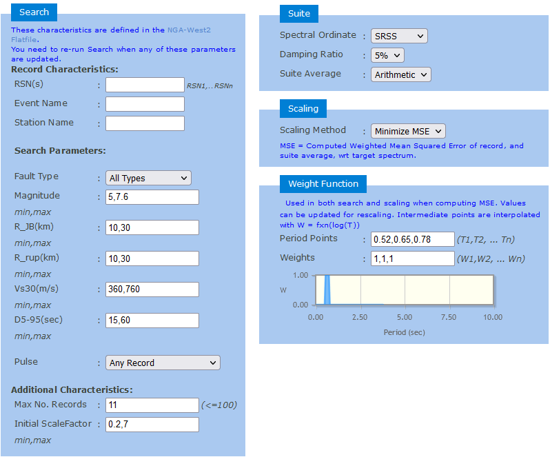
Solution
The PEER website provides the required information in a zipped file, which contains the metadata of the search and results such as latitude, longitude, scaling, significant duration, etc., for each selected record, as well as the spectral results, typically in a CSV file format. In addition, the website also provides each selected record commonly in AT2 file format. For each selected record, there will be three files, one for each directional component of the seismic wave, i.e., North-South (N-S), East-West (E-W), and vertical (V). It is important, but not absolutely necessary, to convert the .csv file to .xlsx in order to read it more efficiently using Python encoding. However, this will depend on the regional configuration of the computer and the delimiter used for the values within the document
# Directory of the .xlsx files
# os.chdir('C:\\Users\\Normando\\OneDrive\\Importante Normando\\Universidades\\PUCE\\14. Semestre Febrero 2022 - Junio 2023\\Diseño Sismoresistente Q210 GR1\\PEERS')               # PC Directory
# directory2 = 'C:\\Users\\Normando\\OneDrive\\Importante Normando\\Universidades\\PUCE\\14. Semestre Febrero 2022 - Junio 2023\\Diseño Sismoresistente Q210 GR1\\PEERS'            # PC Directory
os.chdir('C:\\Users\\norma\\OneDrive\\Importante Normando\\Universidades\\PUCE\\14. Semestre Febrero 2022 - Junio 2023\\Diseño Sismoresistente Q210 GR1\\PEERS')                # Laptop Directory
directory2 = 'C:\\Users\\norma\\OneDrive\\Importante Normando\\Universidades\\PUCE\\14. Semestre Febrero 2022 - Junio 2023\\Diseño Sismoresistente Q210 GR1\\PEERS'             # Laptop Directory
directory2
filenames = glob.glob(directory2 + "\*.xlsx")               # read all the files with extension .xlsx i.e. excel, in the current directory.
DataPEER = pd.read_excel(filenames[0])                      # Selecting the corresponding Excel file, in this case, there is only one file in the directory.
DataPEER
| Unnamed: 0 | Unnamed: 1 | Unnamed: 2 | Unnamed: 3 | Unnamed: 4 | Unnamed: 5 | Unnamed: 6 | Unnamed: 7 | Unnamed: 8 | Unnamed: 9 | ... | Unnamed: 24 | Unnamed: 25 | Unnamed: 26 | Unnamed: 27 | Unnamed: 28 | Unnamed: 29 | Unnamed: 30 | Unnamed: 31 | Unnamed: 32 | Unnamed: 33 | |
|---|---|---|---|---|---|---|---|---|---|---|---|---|---|---|---|---|---|---|---|---|---|
| 0 | PEER Ground Motion Database | Time Series Search Report -- NGA-West2 -- 202... | NaN | NaN | NaN | NaN | NaN | NaN | NaN | NaN | ... | NaN | NaN | NaN | NaN | NaN | NaN | NaN | NaN | NaN | NaN |
| 1 | NaN | NaN | NaN | NaN | NaN | NaN | NaN | NaN | NaN | NaN | ... | NaN | NaN | NaN | NaN | NaN | NaN | NaN | NaN | NaN | NaN |
| 2 | NaN | NaN | NaN | NaN | NaN | NaN | NaN | NaN | NaN | NaN | ... | NaN | NaN | NaN | NaN | NaN | NaN | NaN | NaN | NaN | NaN |
| 3 | -- Summary of PEER Ground Motion Database Sea... | NaN | NaN | NaN | NaN | NaN | NaN | NaN | NaN | NaN | ... | NaN | NaN | NaN | NaN | NaN | NaN | NaN | NaN | NaN | NaN |
| 4 | Magnitude Min: | 5.5 | NaN | NaN | NaN | NaN | NaN | NaN | NaN | NaN | ... | NaN | NaN | NaN | NaN | NaN | NaN | NaN | NaN | NaN | NaN |
| ... | ... | ... | ... | ... | ... | ... | ... | ... | ... | ... | ... | ... | ... | ... | ... | ... | ... | ... | ... | ... | ... |
| 275 | 12 | 0.005975 | 0.004543 | 0.00127 | 0.002386 | 0.006741 | 0.00176 | 0.001263 | 0.001702 | 0.000673 | ... | 0.00181 | 0.005678 | 0.004559 | 0.00133 | 0.003119 | 0.00753 | 0.00183 | 0.005933 | 0.007749 | 0.00348 |
| 276 | 13 | 0.005108 | 0.003791 | 0.00101 | 0.002016 | 0.005721 | 0.0014 | 0.001014 | 0.001527 | 0.000575 | ... | 0.00139 | 0.00446 | 0.0041 | 0.00102 | 0.002558 | 0.006514 | 0.0015 | 0.004718 | 0.006213 | 0.00288 |
| 277 | 14 | 0.004357 | 0.003106 | 0.000824 | 0.001715 | 0.00488 | 0.00114 | 0.00083 | 0.001357 | 0.000496 | ... | 0.00124 | 0.00358 | 0.003408 | 0.000832 | 0.002056 | 0.005512 | 0.00124 | 0.00385 | 0.00496 | 0.00237 |
| 278 | 15 | 0.003722 | 0.00253 | 0.000686 | 0.001469 | 0.00419 | 0.000946 | 0.000692 | 0.001198 | 0.000432 | ... | 0.00108 | 0.002937 | 0.00276 | 0.000683 | 0.001684 | 0.004583 | 0.00109 | 0.003218 | 0.004508 | 0.00195 |
| 279 | 20 | 0.001828 | 0.001173 | 0.000346 | 0.000757 | 0.002165 | 0.000455 | 0.000348 | 0.000649 | 0.000239 | ... | 0.000496 | 0.001411 | 0.001432 | 0.000323 | 0.000873 | 0.001817 | 0.000592 | 0.001667 | 0.002966 | 0.001 |
280 rows × 34 columns
Therefore, to obtain the relevant data, it is crucial to identify the search parameters that were used during the data collection process. Once these parameters have been determined, the data can be extracted from the corresponding location in the Excel document. It should be noted that the accuracy of the extracted data will depend on the correctness of the search parameters used.
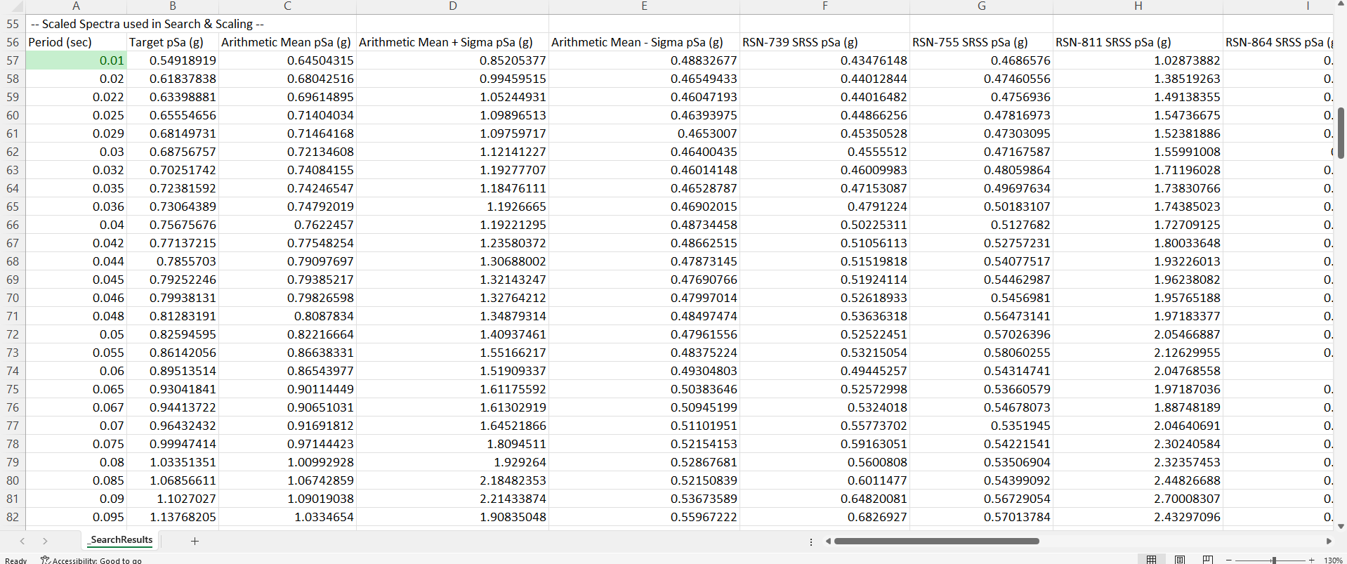
row_in = 55
row_fin = 165
T = DataPEER.iloc[row_in:row_fin, 0]
final_row = np.where(T == 4)[0][0]
T = np.array(T)
Specs = DataPEER.iloc[row_in:row_fin, 1:]


fig, ax = plt.subplots(figsize=(16/1.5, 9/1.5))                                                                 # Create a figure and an axes object

ax.plot(T, Specs, color=(0, 0, 0), marker='+', markersize=0, markerfacecolor='w',                               # Plot the Elastic Acceleration Response Spectra
 markeredgewidth=0, linewidth=1.0, alpha=0.3,linestyle = '-')
ax.plot(T, DataPEER.iloc[row_in:row_fin, 1], color=(0, 0, 0), marker='+', markersize=0, markerfacecolor='w',    # Plot the Elastic Acceleration Response Spectra
 markeredgewidth=0, linewidth=2.0, alpha=1,linestyle = '-',label= f'Target, Sa_elastic')
ax.plot(T, DataPEER.iloc[row_in:row_fin, 2], color=(0, 0, 1), marker='+', markersize=0, markerfacecolor='w',    # Plot the Elastic Acceleration Response Spectra
 markeredgewidth=0, linewidth=2.0, alpha=1,linestyle = '-',label= f'Arithmetic Mean pSa')
ax.plot(T, DataPEER.iloc[row_in:row_fin, 3], color=(0, 0, 1), marker='+', markersize=0, markerfacecolor='w',    # Plot the Elastic Acceleration Response Spectra
 markeredgewidth=0, linewidth=1.0, alpha=1,linestyle = '--',label= f'Arithmetic Mean + Sigma pSa')
ax.plot(T, DataPEER.iloc[row_in:row_fin, 4], color=(1, 0, 1), marker='+', markersize=0, markerfacecolor='w',    # Plot the Elastic Acceleration Response Spectra
 markeredgewidth=0, linewidth=1.0, alpha=1,linestyle = '--',label= f'Arithmetic Mean - Sigma pSa')

ax.set_xlim([T[0], T[final_row]])                                                                               # Set the x-axis limits from 0 to the maximum value in Period
plt.title('SCALED SPECTRA', fontsize=10, color=(0, 0, 1))                                                      # Set the title of the plot to 'UHS'
plt.xlabel('Period (T) [s]', rotation=0, fontsize=10, color=(0, 0, 0))                                          # Set the x-axis label to 'Period (T) [s]'
plt.ylabel('Max Response Acceleration (Sa) [g]', rotation=90, fontsize=10, color=(0, 0, 0))                     # Set the y-axis label to 'Max Response Acceleration (Sa) [g]'
legend = plt.legend(fontsize=10)                                                                                # Add a legend to the plot with a font size of 10
legend.get_frame().set_edgecolor('none')                                                                        # Remove the frame from the legend
ax.grid(which='both', axis='x', alpha=0.5)                                                                      # Add gridlines to both the x and y axis
plt.show()